
Making Aging Analysis Reports Using Excel – How To
Making Aging Analysis Reports Using Excel – How To
If you are new to this analysis tool and don’t know what it does I strongly recommend reading the above mentioned explanation as only then you will grab the concept of what we are going to do and why we are going to do.

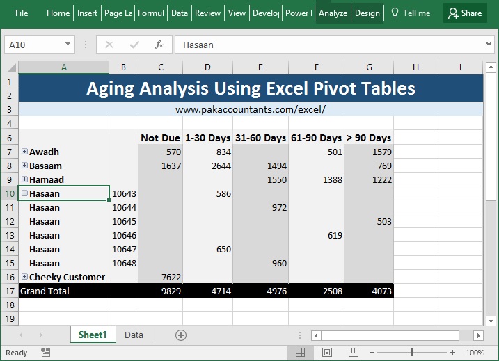
This is what our end result at the end of this tutorial looks like:
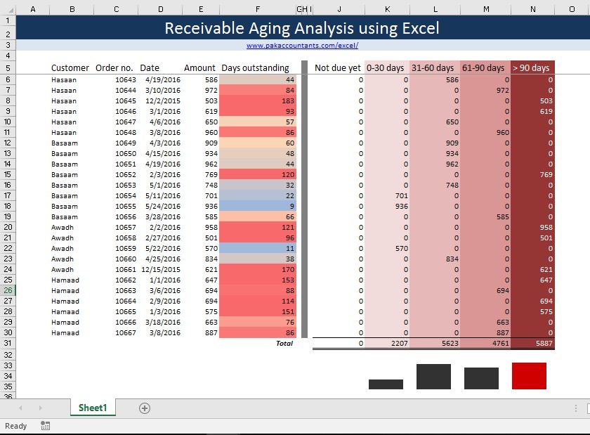
In very few words and if I try to define aging analysis in context of receivables or debtors, then it is an analysis that helps me determine when certain sales invoices are falling due. And more importantly since how long a certain receivables are outstanding. First aspect helps me determine expected cash flows. Second helps me determine where recovery department must concentrate its efforts.
Excel Tutorial Workbook
Download this example workbook that provides you with the necessary data and to apply the concepts learnt in this tutorial
A dash at the data and requirements
Open up the workbook you downloaded and its a fairly simple data consisting of four very fragrant debtors. Each has several invoices against its name with different due dates. We want to classify invoices as follows:
- Not due: The invoices which that has not fallen due yet
- 0-30 days: The invoices that are past due for days between 1 to 30 days.
- 31-60 days: The invoices that are past due for days between 31 to 60 days
- 61-90 days: The invoices that are past due for days between 61 to 90 days
- >90 days: the invoices that are past due for more than 90 days.
Understanding the approach – Aging Analysis Reports in Excel
So it seems simple and it is simple if you know how to go about IF function and how to make multiple IF statements using AND function. Its all part of today’s discussion.
But as I always like to raise the bar a little higher than requirement so I will going one step further and will do:
- aging analysis using the slabs give above i.e. not due, 0-30, 31-60 etc.
- compute the number of days since the invoice is outstanding
So lets get started!
Watch a walkthrough OR continue reading for something additional!
You can either watch the following video on aging analysis in Excel to prepare basic aging analysis report OR continue reading to learn additional techniques involving conditional formatting and sparklines!
Adding column headers
We need to add few headings here to accommodate our requirement. So in cell
- E1 type: Days outstanding
- F1 type: Not due
- G1 type: 0-30 days
- H1 type: 31-60 days
- I1 type: 61-90 days
- J1 type: >90 days

Giving Data Wings Meaning! – Number crunching Time!
Step 1: In cell E5 put the following formula press Enter:
=IF(TODAY()>C5,TODAY()-C5,0)
This formula checks that if today’s date is later or greater than the date mentioned in cell C5 the deduct today’s date from the date in cell C2 to calculate the number of days. However, if today’s date is earlier than the date in C5 then put 0 as a result.
Step 2: To apply the same formula in order to calculate the days for all the invoices simple double click the fill handler and it will populate the cells immediately of column E.

Giving Data even more meaning!
Although we have calculated number of days and manager can easily sort and filter the column to find the invoices exceeding certain number of days. But using conditional formatting feature in Excel we can create a sort of heatmap to show values with long outstanding period as red and the ones that are in favourable time range as blue or similar color. By adding colors to the data, its much easier to identify and focus on important aspects of data. Follow these steps to accomplish it
Step 1: Select the values in Column E that you just calculated using formula. You can make selection with mouse or using keyboard shortcuts. To learn how to select using shortcuts read this: 40+ Excel navigational shortcuts to make accounting job super efficient
Step 2: Go to Home tab > Styles group > click the conditional formatting drop down > click new rule. A new dialogue box will appear
Step 3: Make sure the first option is selected. From the format style drop down selection menu select 3-color scale. This will enable three shades possibility.
Step 4: From type drop-down menu select number option under each of the three categories i.e. minimum, midpoint and maximum.
Step 5: Set the values as following:
- minimum: 0
- midpoint: 60
- maximum: 90
Step 6: Select the colors you like for minimum, midpoint and maximum values. I chose blue for minimum, beige for midpoint and red for maximum. You can select any that suits your need and liking. Click OK
Joys!!! now you can instantly see what invoice needs immediate attention. (It seems this company’s recovery department is doing nothing at all!!!)
Aging Analysis Report in Excel! – Finding the lazy ones!
Now the next part which is our actual requirement i.e. to have the ageing or aging or aged analysis of each of the invoices. Follow along:
Step 1: In cell F5 put the following formula:
=IF(E5=0,D5,0)
This formula checks that if value in cell E5 is not equal to zero then fetch the value in cell D5 as this column is “not due” and this way the value of invoice will be inserted here as “zero” in cell E5 means it hasn’t even fallen due.
Step 2: In cell G5 of column 0-30 days put the following formula:
=IF(C5<TODAY(),(IF(TODAY()-C2<=30,D5,0)),0)
The above formula is an example of nested IF statements in which we basically have IF function within IF function. In words the above formula will be said as follows:
If date in cell C5 is earlier then the date than today then check if the difference between today and date in cell C5 is less than or equal to 30 days. If it is less than or equal to 30 days then fetch the value from cell D5. If not equal or less than 30 days then put 0. And also if today is later than the date in cell C5 then put zero.
Once the formula is in place. Press Enter and double click the fill handle to apply the same formula down the column covering all the invoices. Following animation helps

Step 3: Next column is of 31-60 days. This is a bit challenging as we two conditions to meet check if the invoice is past due for days upto 60 days but more than 30 days. In other words it must exclude the invoices that has fallen due for in last 30 days. If we don’t add second condition then it will include those invoices as well that have fallen in last 30 days as when I ask it for all the invoices that has fallen due in last 60 days, the invoices fallen due in last days also fall in this criteria. So I have to tell Excel to exclude such invoices. To do this put the following formula in cell K5:
=IF(AND(TODAY()-$C5<=60,TODAY()-$C5>30),$D5,0)
The above formula is an example of multiple IF statements or multiple criteria where each criteria is joined using AND function. AND function does literally the same thing as the and does in language. So the above formula will be read like this in plain English:
If difference between today’s date and the date in cell C5 is less than or equal to 60 days AND the difference between today’s date and the date in cell C5 is greater than 30 days than fetch the value from cell D5 otherwise put 0.
This can also be said like this; fetch the value from cell D5 if both of the following conditions are met:
- if difference between today’s date and the date in cell C5 is less than or equal to 60 days; AND
- if the difference between today’s date and the date in cell C5 is greater than 30 days
Once the formula is in place press Enter and double click or drag the fill handle to apply the formula to rest of the invoices.
Step 4: Next is 61-90 days column and on the same concept as used in above step we will adjust the formula to find us the right invoices. Following is the formula that you will put in cell I2. Press Enter and drag the fill handle to populate the column with formula:
=IF(AND(TODAY()-$C5<=90,TODAY()-$C5>60),$D5,0)
Step 5: Under column >90 days put the following formula in cell J5:
=IF(TODAY()-$C5>90,D5,0)
This is a simple formula which is checking if the difference between today’s date and the date in cell C5 is greater than 90 days then fetch the value from cell D5 otherwise insert 0. Double click the fill handle to paste the same formula down the range.
Hurrah!!! You have completed the aging analysis and now you can see what invoice falls under what category. Well job done! Now you can sum the values of invoices to calculate the invoices that are falling in each category. To quickly do that select cell F30 to J30 and hit Alt+= and in the blink of an eye you have the totals! Just excelling at excel every moment. Two thumbs up!!! 

Bonus Tip: Adding Spark to the data! – Sparklines!
Yes we do have total numbers of invoices under each category. But it always good to see the data instead of reading it. To add a little spark to the totals lets blend the eye-candies using Excel’s sparklines feature!
Step 1: Select the area within cell F32 and J 34. Go to home tab > Alignment group > Click merge and center button.
Step 2: Select the merged area you created and go to Insert tab > Sparklines group > click column button. A dialogue box will open. Click once inside the data range and then select the totals you did for each category of invoices. Click OK.
You get a nice looking graph made up for you instantly and that is sitting right inside cells! How sparky is that! If you change the data the sparklines graph will update automatically.
To read more about sparklines please check out this page for full listing of articles on sparklines and their use
Lucky me! Common sense knocked the door!
Well yes I must admit that my brain really had tough day today and probably the marriage with common sense is going through bad patch. But it felt pity and did pulled some neurons and made me think about another way to do aging analysis.
Look at the formula I suggested above. Basically in those formulas I used today’s date and the date in cell C5. I completely bypassed the days I calculated!!! I could have used the days I calculated and building formula would have been even more easier. But I leave that for you to do as I am a person who assume that if you understand a thing through difficult route you must be able to do it the easy way easily! 
Download Fully Worked Excel file
You can download the fully worked file free of cost but if you like the effort and gained something valuable then you can set the price whatever you deem fit and pay. If you want to download it for free then simply set the price to “0”. Enjoy!
Download NowHomework!
Well yes I do have one other homework for you. Above is the example of receivables aging analysis. Now try to make the creditors aging analysis in which you have determine which invoice is falling due in next specific time lapses. To do this assignment download this file.
Next step – Aging analysis using Excel Pivot tables
In the above tutorial we used formula approach to get the job done. But we can do this and much more using pivot tables. To learn how to do aging analysis using pivot tables check out: Making Aging Analysis Reports using Excel Pivot Tables – How To
 Loved it? Pin it!
📤How to Download ebooks: https://www.evba.info/2020/02/instructions-for-downloading-documents.html?m=1


Leave a Comment