Making Profit and Loss Statements in Excel using Pivot tables

 Being an accountant myself trust me I hate numbers and all that journals and “T” accounts. But its necessary to get to much meaningful financial statements like Statement of Financial Position (Balance sheet) and Profit and loss Statement (Income statement).

Excel’s ability to store data in rows and columns is exceptionally flexible and Pivot tables capitalize on it beautifully. Today we will take a sample data and learn how to make a profit and loss statement in minutes (if not seconds).

Potential data problems

IF we intend to make profit and loss statement using pivot table then data has to be structured in a certain way i.e. “columnar”. In pivot tables, each column and its header will become a criteria that can be used to produce a report. If your data is not arranged in meaningful columns then even pivot table will be of less help.

Two main problems we often encounter are:

Data is not columnar. To manage this situation we can either use formula method, power query method, or even use pivot tables method to structure data. Check the links to learn more about these methods.

Data is scattered in different worksheets, workbooks or files of different programs. To solve this problem we can use simple copy/paste, LOOKUP functions or again employ power query to combine data using different tools available. One of such tool append data using power query.

Once these issues are resolved we can continue with pivot tables to generate profit and loss reports easily.

Emphasis of fact

For the purpose of this tutorial I am using the same data set that I have used in other connected tutorials as I believe it will make much more sense.

Here I am listing the tutorials in the order that should be read and summarizing what is achieved in them:

1. Normalize data either using power query, pivot table or formulas
2. Combine scattered data in one table using append tool in power query

The tutorial file that I am providing with this tutorial is actually what we have after we had it normalized and appended.

Download Excel Tutorial Workbook

To better understand the steps discussed in this tutorial download this Excel workbook that provides you the sample data necessary to run through the process of preparing profit or loss statements using pivot tables

Watch the walkthrough video or continue reading!

Making your first P&L Statement in Pivot tables

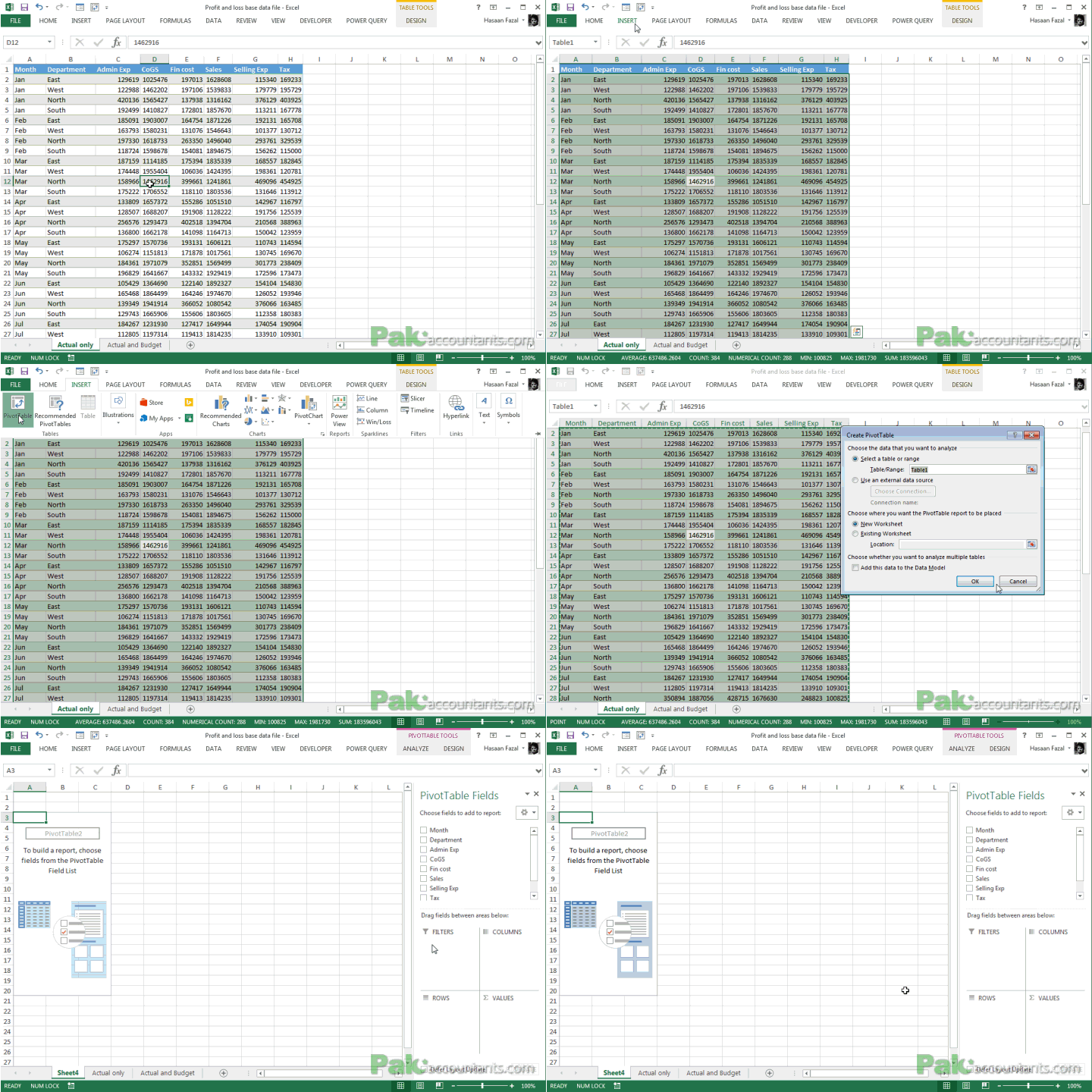
Step 1: Download and open the tutorial workbook. Go to Actual only worksheet. Select the range and go to Insert tab > click pivot tables and click OK button. A new worksheet will be inserted with report generation capability.

Step 2: Move the fields in the following order to values quadrant one after the other:

1. Sales
2. CoGS
3. Admin Exp
4. Selling Exp
5. Fin Cost
6. Tax

Step 3: You will see that value field is inserted in the columns quadrant automatically. Drag it to rows column.

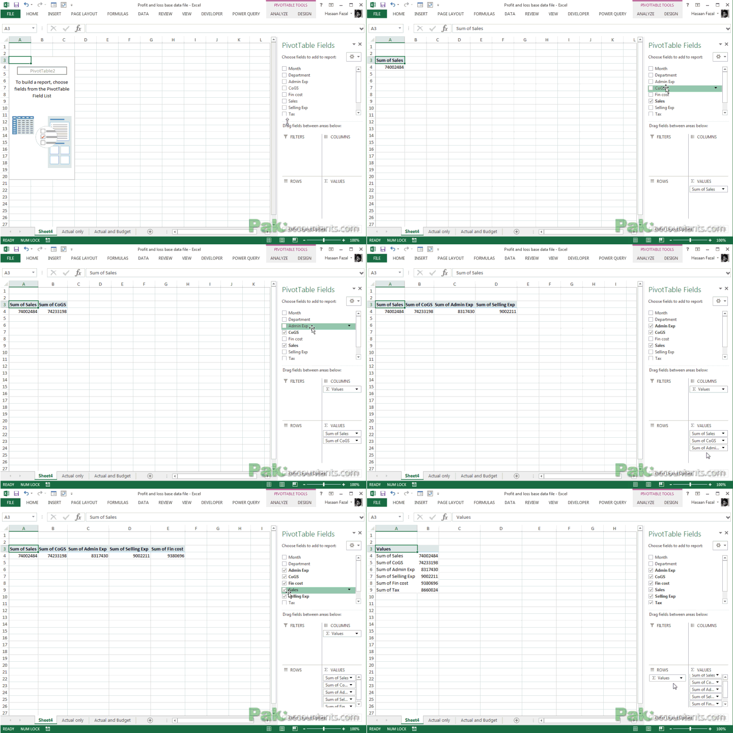
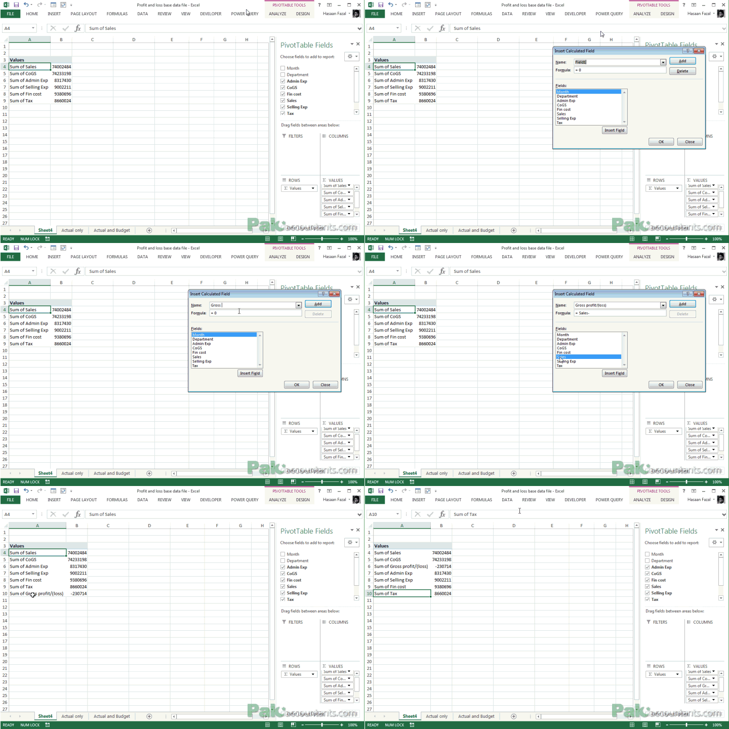
Step 4: Now that we have the figures in place we need subtotals for gross profit or loss, operating profit or loss, profit before tax and profit after tax. To get this done we will take help of calculated fields inside pivot tables.

Having an active cell inside pivot table, click analyze tab > calculations group > click Fields, Items, Sets > click Calculated field. In the name field type “Gross profit/(loss)”. Have the cursor in formula bar after “=” sign and double-click “sales” hit minus “-” key on the keyboard and then double click “CoGS” field. Click OK button. Move the newly inserted field under CoGS field.

Step 5: Add another calculated field for operating profit/loss calculation and move it to appropriate place. Following animation will help

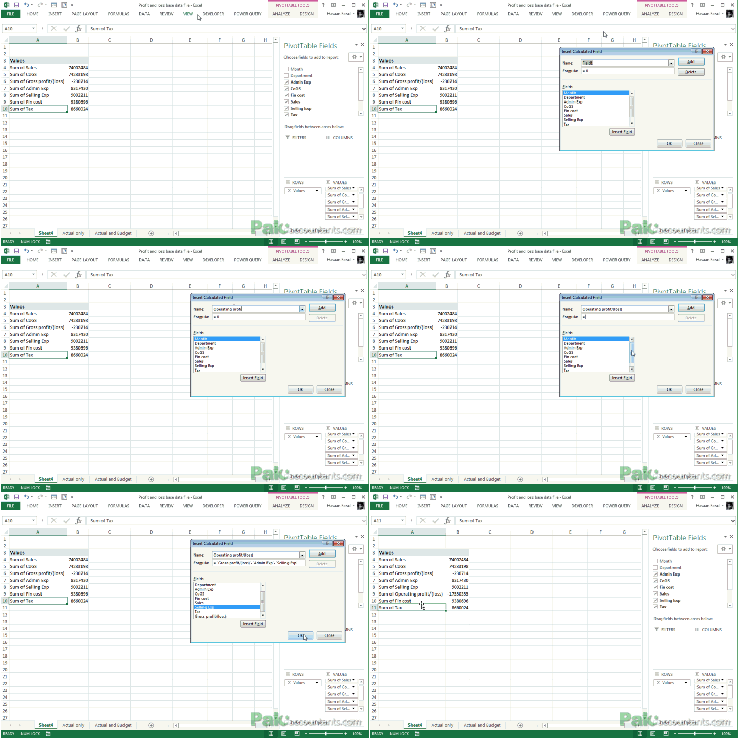
Step 6: Add another calculated field for Profit/(loss) before tax. And after that final field will be regarding Profit/(loss) after tax.

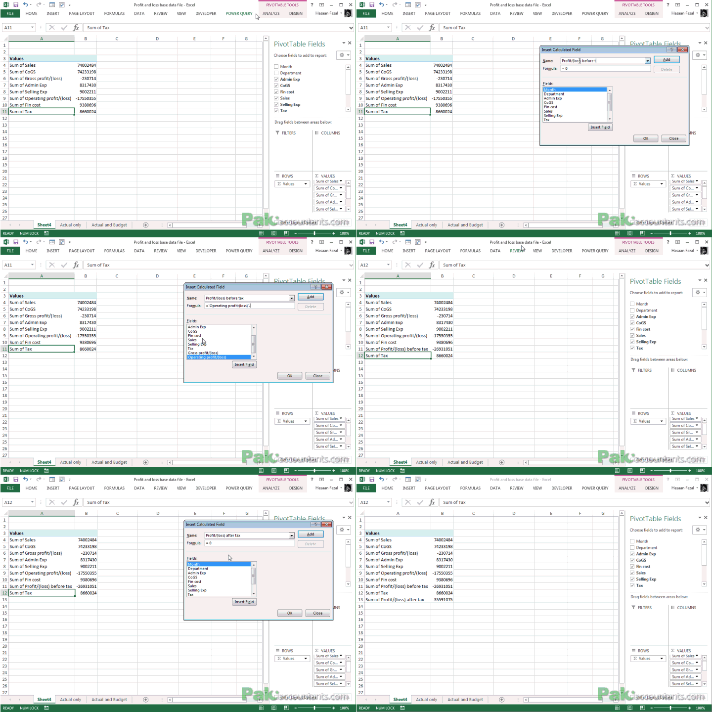
Once these calculated fields are added, we are now ready to format the profit and loss statement.

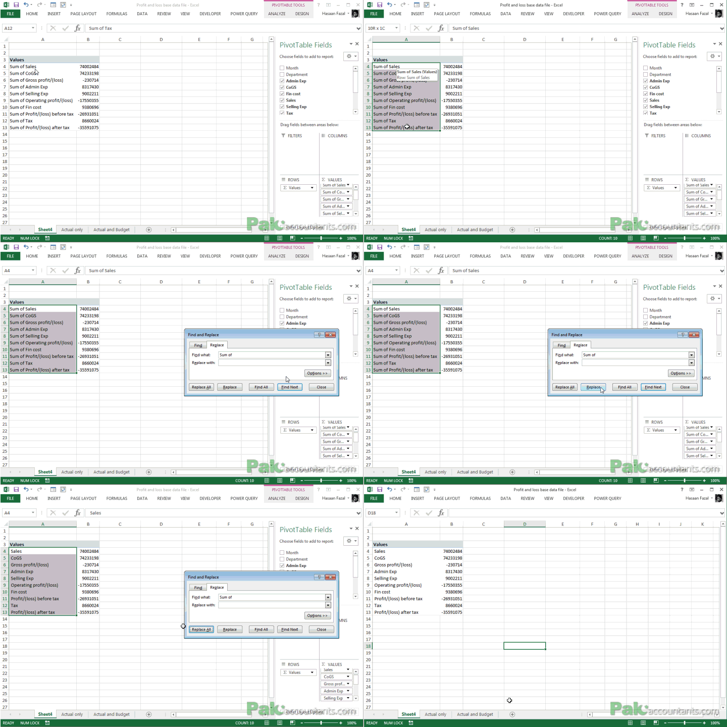
Step 7: See the “Sum of” with all the fields in the start. That’s ugly! Select the first column and hit Ctrl+H. In “Find what” field type Sum of and leave “Replace with” field empty. Click OK and boom!

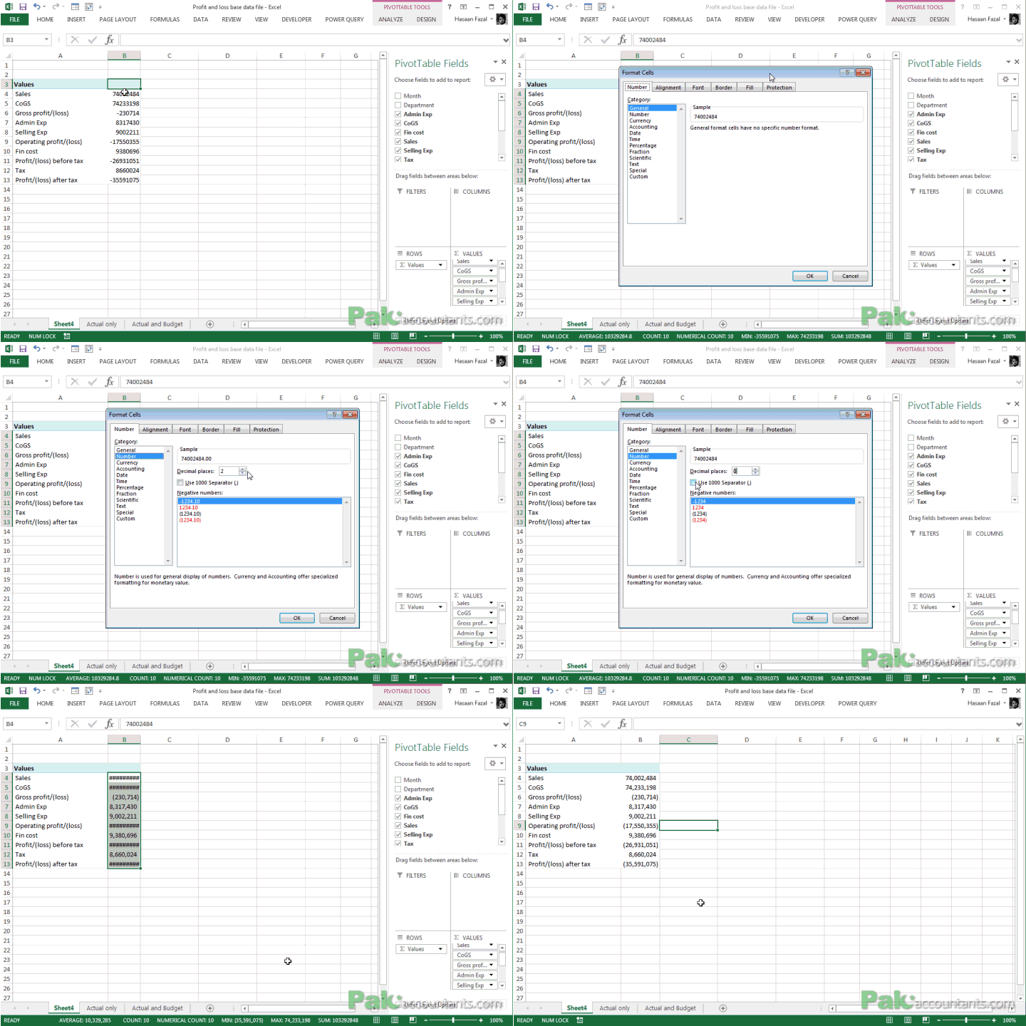
Step 8: Select the column containing values and hit Ctrl+1 to open Number format options window. On the left hand side click “number”. Check mark “1000 separator” option. Also select the appropriate negative number format. Click OK to update the formats

Step 9: Now to make it more understandable we need to add few lines to emphasize subtotals like gross profit, operating profit, profit before tax and profit after tax. I used borders to add the visual ease.

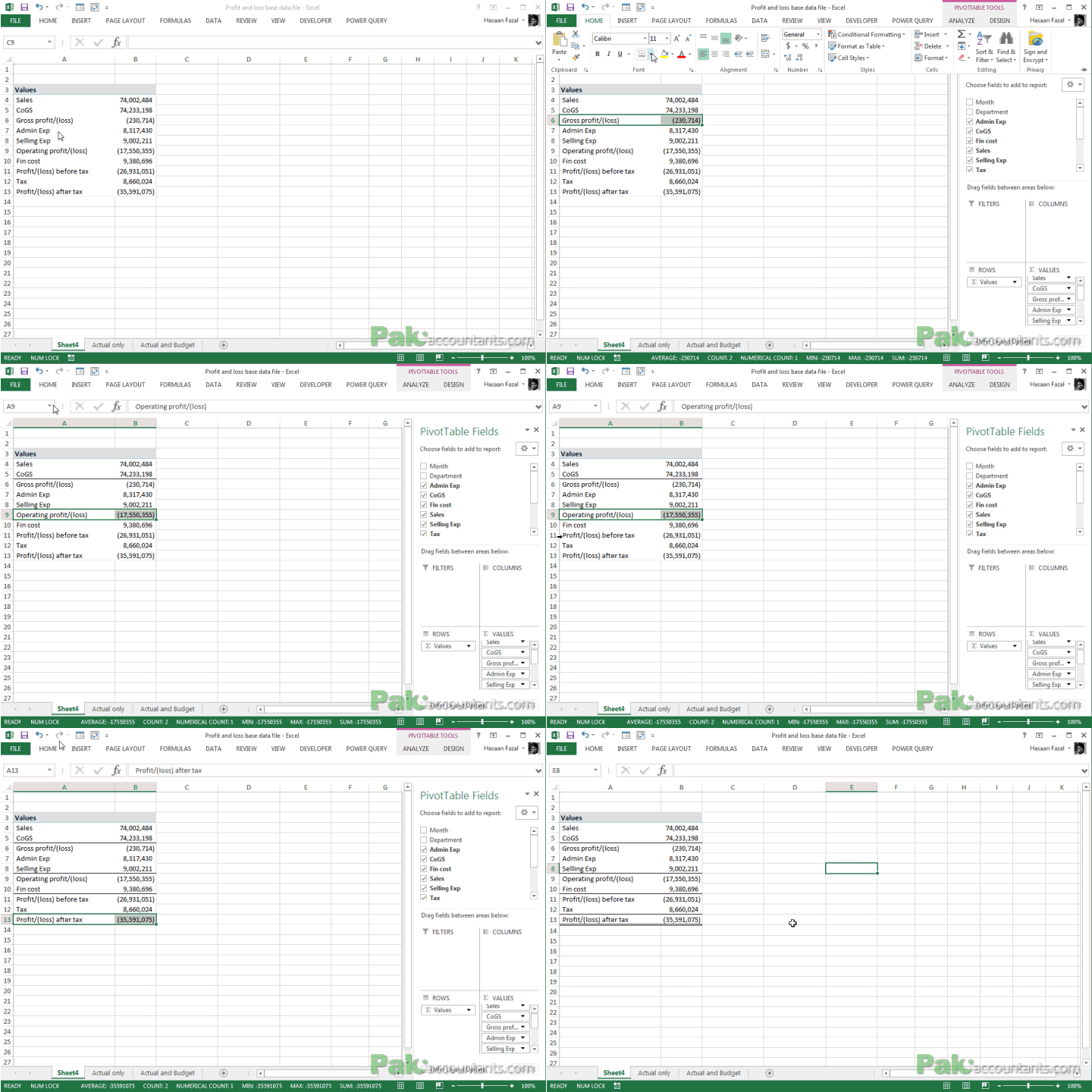
So here you have a very basic profit or loss statements all ready in few minutes. Pivot tables has really saved us from many different LOOKUP functions and conditional SUM formulas.