How to Use the TAKE and DROP Functions in Excel

Learn how to precisely extract and manipulate your data, making Excel work smarter for you.

Readers like you help support MUO. When you make a purchase using links on our site, we may earn an affiliate commission. Read More.

When working with your dataset in Microsoft Excel, there are occasions when you need to analyze only a portion of the data. Thankfully, Excel provides the TAKE and DROP functions for situations like this.

TAKE and DROP allow you to include or exclude a portion of an array in your selection. Let's start by defining these functions and then explore how to use them in Excel.

What Is the TAKE Function in Excel?

The TAKE function in Excel extracts a specified number of rows and columns from an array. The syntax of the TAKE function is:

=TAKE(array, rows, [columns])

Here's what each parameter signifies:

• Array: Refers to the source array from which you wish to extract rows or columns.
• Rows: Indicates the number of rows to extract. A negative number takes rows from the end.
• Columns: Indicates the number of columns to extract. A negative number also takes columns from the end.

What Is the DROP Function in Excel?

On the other hand, the DROP function in Excel excludes specific rows and/or columns from an array or range of cells. The syntax of the DROP function is:

=DROP(array, rows, [columns])

The parameters for the DROP function are similar to those in the TAKE function:

• Array: Refers to the source array from which you wish to remove rows or columns.
• Rows: Indicates the number of rows to remove. A negative number removes rows from the end.
• Columns: Indicates the number of columns to remove. A negative number removes columns from the end.

The TAKE and DROP functions work with arrays, and they output arrays as well. Since they always output arrays, there's no need to mark them as array formulas in Excel. For the same reason, you might encounter the #SPILL error in Excel when using TAKE and DROP.

TAKE and DROP are available in Excel for Microsoft 365, Excel for Microsoft 365 for Mac, and Excel for the web. However, older versions of Excel do not have these functions.

How to Use the TAKE Function in Excel

There are infinite Excel scenarios where TAKE might come in handy. Let's take a look at a few examples.

1. Extract the Top Five Rows of Your Data

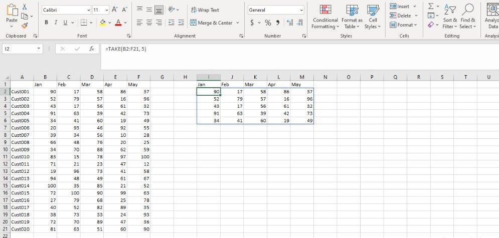
Suppose you have a worksheet containing a list of products and their prices over the past few months. If you want to extract only the first five rows of the data, you can use the TAKE function instead of copying the data.

Here's how you can do that:

1. Select the cell where you want to use the TAKE function.
2. In the formula bar, enter the formula below.

   =TAKE(B2:F1, 5)

3. Press Enter.

This formula will retrieve the first five rows within the data range B2:F1 and return the output.

2. Extract the First Column of Your Data

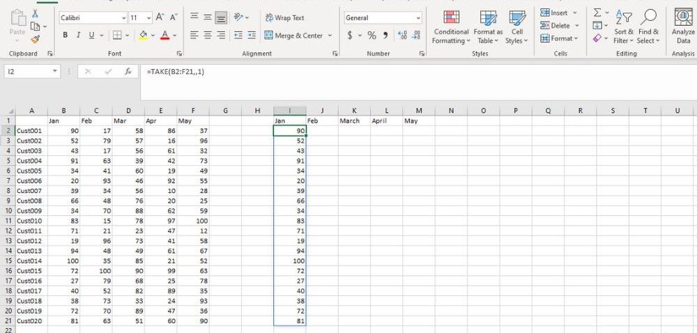
Let's say you want to retrieve only the first column in the same dataset. To do this with the TAKE function, you need to leave the row parameter empty and only specify the column:

=TAKE(B2:F1,,1)

This formula will retrieve the first column from the B2:F1 data range. Since we didn't specify any value for the row parameter in our formula, every row in the first column is included in the output.

How to Use the DROP Function in Excel

You can use the DROP function to exclude unwanted rows and columns from your data. The syntax for the formulas is similar to the TAKE function. Let's see how the DROP function works in Excel.

1. Exclude the Last Ten Rows of Your Data

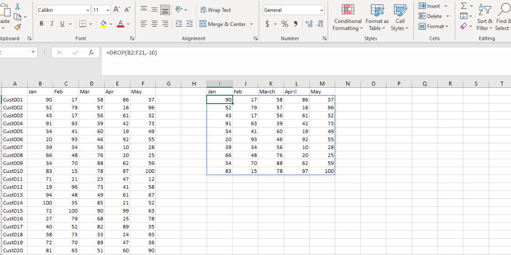
Suppose you want to create a data view of your worksheet that shows everything except the last ten rows. Here is the formula you can use to achieve this:

=DROP(B2:F21,-10)

This formula will exclude the last ten rows in the B2:F1 data range. This is because we specified -10 as the row parameter of data.

2. Exclude the Last Column of Your Data

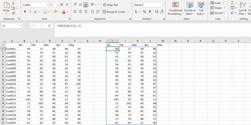
You can use the formula below to trim down the last column of your data with DROP:

=DROP(B2:F21,,-1)

In this example, the DROP function will return the values that fall within the range B2:F1 while excluding the last column.

Combining the TAKE and DROP Functions With Other Excel Functions

The true magic of Excel happens when you combine different functions together. For instance, if you need to feed a specific part of an array to a function, you can combine it with TAKE or DROP instead of writing out the data range.

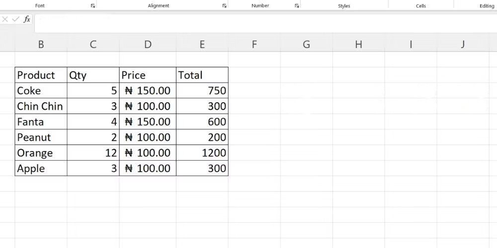
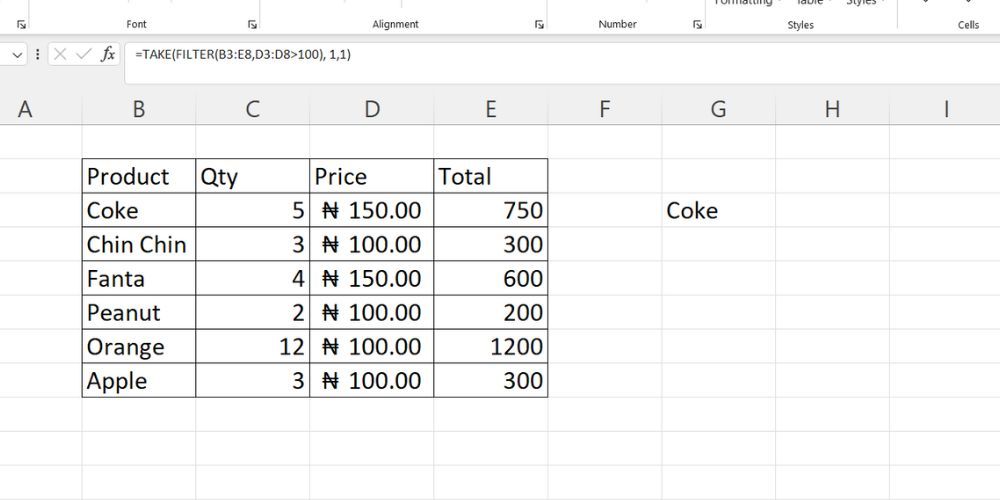
Suppose you have a table of some items and their details and want to output the first item that costs above N100. You can use TAKE in combination with the FILTER function in Excel to do this. Here's the formula to do that:

=TAKE(FILTER(B3:E8,D3:D8>100), 1,1)

Let's break this formula down. The FILTER function gets all rows with prices above N100 within the range. The formula for this is as follows:

=FILTER(B3:E8,D3:D8>100)

Next, the formula feeds the results from FILTER to the TAKE function. Specifying both the row and column arguments as 1 retrieves only the value in the filtered data's first row and column.

Take and Drop Data in Your Sheet

Excel's TAKE and DROP functions offer a powerful way to extract and manipulate specific data in your worksheets. Understanding their syntax and usage allows you to efficiently manage and analyze your Excel data, especially when combined with other functions.