03 Types of Excel Cell Reference: Relative, Absolute & Mixed

An Excel Cell Reference is a cell address that identifies a cell’s location in the worksheet, based on its column letter and row number.

For example, A1 refers to the cell at the intersection of column A and row 1; A2 refers to the second cell in column A and row 2. 

Using Excel cell references is advantageous because if the values in the referenced cells are changed, the formula result automatically updates using the new values. Thus, using a cell reference rather than values in a cell gives more flexibility in a worksheet.

For example, the formula =A1+A2 adds the values in cells A1 and A2. If cell A1 contains the number 10 but is later changed to 20, the formula that references cell A1 updates automatically. 

The same principle applies to a cell that contains a formula and is referenced in another formula.

 Excel Cell reference is broadly used in formulas (a user-defined calculation), functions (pre-defined formulas in Excel such as SUM, VLOOKUP, HLOOKUP, COUNTIFS, SUMIFS, etc.), charts, and other Excel commands.

For example, =A1+B1 has been just a formula, but =SUM(A1:B1) is a formula containing a function (i.e., SUM).

There are basically three types of cell references in Excel:

(01) Relative cell reference

(02) Absolute cell reference

(03) Mixed cell reference

I. WHAT IS A RANGE REFERENCE IN EXCEL?

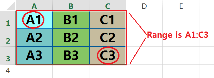
A range reference is a continuous block of two or more cells to make a range. It is represented by the address of the upper-left cell and the lower right cell separated with a colon.  

For example, the range A1:C3 having 9 cells from A1 to C3.

II. WHAT ARE REFERENCE STYLES IN EXCEL?

There are two Excel cell reference styles:

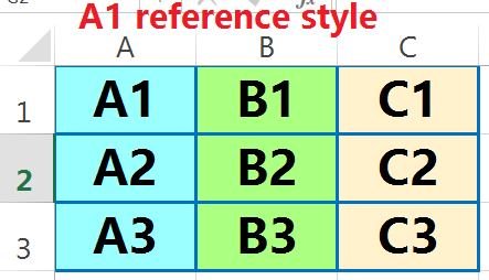
(01) A1 REFERENCE STYLE IN EXCEL

The A1 reference style is the default style in Excel. In this style, columns are defined by letters and rows by numbers, i.e. A1 defines a cell locates in column A and row 1.

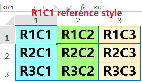
(02) R1C1 REFERENCE STYLE IN EXCEL

In the R1C1 reference style, both rows and columns are identified by numbers, i.e. R1C1 designates a cell in row 1, column 1. Here “R” defines “Row” and “C” defines “Column”. At a glance, the below screenshots illustrate both the A1 and R1C1 reference styles:

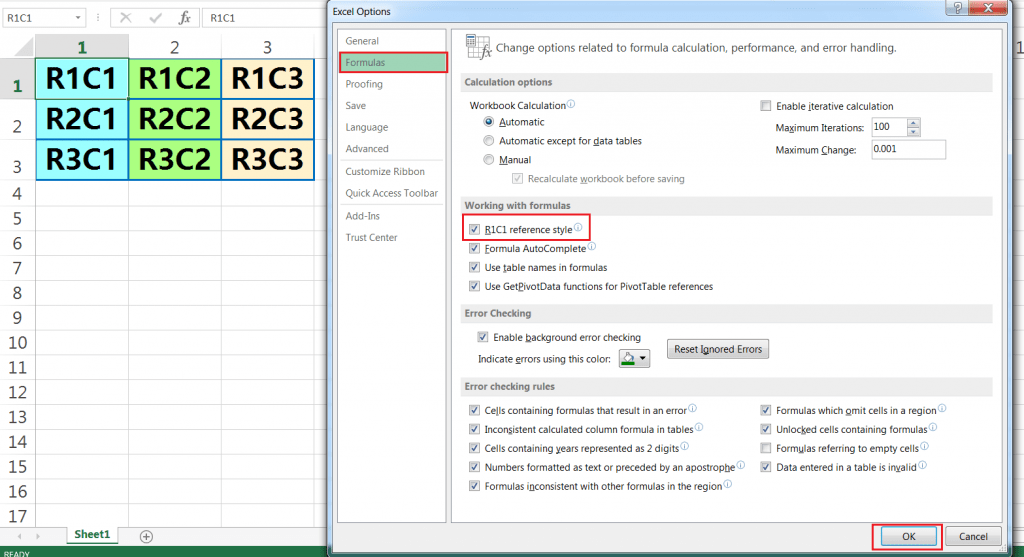
HOW TO SWITCH FROM EXCEL A1 REFERENCE STYLE TO THE EXCEL R1C1 REFERENCE STYLE OR VICE VERSA?

To switch from the default A1 reference style to the R1C1 reference style, we go to the top left side corner of excel and click on File ➪ Options ➪ Choose Formulas (at the left sidebar) ➪ select the R1C1 reference style checkbox (for switching from A1 reference style to R1C1 reference style) or uncheck the box (for switching from R1C1 reference style to A1 style) ➪ Then click OK button. 

III. OVERVIEW OF VALUES, FORMULAS, AND EXCEL CELL REFERENCE 

This tutorial introduces values, formulas and the cell references required to write a formula. 

➢ Values

Values are any numerical data entered in a worksheet. Once values are entered into the worksheet, they can be used in formulas. 

➢ Formulas

Formulas are values, but unlike normal values, formulas contain information to perform a numerical calculation, such as adding, subtracting, multiplying or dividing. For example, a cell with the formula = 10+20 will display the result of the calculation: 30. 

All formulas must start with an equal sign (=). Then need to specify more information for calculation: (1) the values to calculate and (2) the function name(s) or the arithmetic operator(s).

• Functions are frequently used in advanced Excel. Functions are pre-made specialized formulas built into Excel that are used as shortcuts or to perform a wide range of calculations. For example, Excel provides dedicated functions that calculate sums and averages, standard deviations, yields, cosines and tangents, and much more.  

• Operators are the basic symbols used in mathematics: + (plus), – (minus), * (multiply) and / (divide). In Excel, use these in the same way as writing out a math problem. These ingredients are also known as arithmetic operators. 

➢ Excel Cell Reference

An Excel cell reference is a cell address and most formulas are created with references to cells or ranges. These references enable the formulas to work dynamically with the data contained in those cells or ranges. 

For example, if any formula refers to cell B1 and the value in B1 is changed, the formula result changes to reflect the new value. 

If we don’t use the Excel cell references in the formulas, then we must edit the formulas manually every time in order to change the values used in the formulas.  

IV. TYPES OF EXCEL CELL REFERENCE: RELATIVE, ABSOLUTE & MIXED 

A key element of a formula is the Excel cell reference. There are three types of Excel cell references: relative cell reference, absolute cell reference, and mixed cell reference.

Each type of Excel cell reference in a formula plays an important role differently when the formula is copied and pasted to a new location.

(01) RELATIVE CELL REFERENCE

A relative cell reference refers to cells in relation to the cell that contains the formula. When the formula is moved, it references new cells based on their location relative to the formula. A relative cell reference is the default type of Excel cell reference.  

A relative cell reference does not use any dollar sign ($) before the column address or the row address.  When a formula is copied or dragged to another cell or range, relative cell reference changes accordingly.

For example, A1

(02) ABSOLUTE CELL REFERENCE

An absolute cell reference always refers to a specific cell or range of cells, regardless of where the formula is located in the worksheet, even when the formula is copied to any other cell in the worksheet.  The row and column references do not change after copying the formula because the reference is to an actual cell address.      

An absolute reference uses two dollar signs ($) in its address: one for the column letter and one for the row number.

For example, $A$1

(03) MIXED CELL REFERENCE

A mixed cell reference is an Excel cell reference that uses an absolute column or row reference, but not both. Only one of the address parts is absolute.   

A mixed cell reference uses a dollar sign ($) either before the column address or before the row address. It is a combination of relative and absolute references (mixed reference type in excel).

For example, $A1 or A$1

• $A1 –  where the column address is absolute and the row address is relative. When copy and paste the cell to a new location, the column address A remains fixed, but the row number changes with the new location of the pasted cell e.g., $A2, $A3, $A4 so on. 

• A$1 – where the column address is relative and the row address is absolute. Similarly, when copy and paste the cell to a new location, row number 1 remains fixed, but the column address changes accordingly with the new location of the pasted cell e.g., B$1, C$1, D$1 so on.

V. HOW TO CHANGE THE MODE OF EXCEL CELL REFERENCES IN A FORMULA

We must remember that to accommodate any changes in the cell references in Excel, we may need to edit the formula and Excel must be in edit mode. 

The following are some of the ways to get into cell edit mode: 

➢ Double-click the cell, which enables editing the cell contents (vales, formulas, text) directly in the cell. 

➢ Press the F2 key, which enables editing the cell contents directly in the cell. 

➢ Select the cell that we want to edit, and then click on the Formula Bar and edit the cell contents. 

While we are editing cell contents, we can select multiple characters either by dragging the mouse cursor over them or by pressing Shift and navigation keys. 

We can quickly switch a cell reference from relative to absolute or mixed. Rather than retyping the formula in every new cell, select the cell reference or range and then repeatedly press the F4 key, Excel cycles through the different reference types – starting with the relative reference, followed by the absolute reference, then to a mixed reference with an absolute row address, followed by a mixed reference with an absolute column address.  

Excel cell reference switches in this order: C2:F12 ➪ $C$2:$F$12 ➪ C$2:F$12 ➪ $C2:$F12

However, we can manually insert dollar signs ($) in the appropriate positions of the cell address. 

VI. HOW TO USE EXCEL CELL REFERENCES IN FORMULAS

Most of the formulas work with the help of references to cells or ranges. These references enable the formulas to work dynamically with the data contained in those cells or ranges. 

In the given figure, using the COUNTIFS function in cell F3 to get the count value based on two criteria – (i) Country name and (ii) Priority scope.

The Syntax of the COUNTIFS function is:

=COUNTIFS(criteria_range1, criterion1, [criteria_range2, criterion2]…and so on)

The formula is written based on the above syntax

=COUNTIFS(C3:C20,E3,B3:B20,F2)

This formula uses Excel relative cell reference.

Copy the formula to the entire selected range with the ‘Formulas and number formats’ option in the Paste Special dialog box.

As the formula uses relative cell reference, therefore when the formula is copied in the cells or ranges, the references adjust in a relative manner. As a result, formula criteria are not matched to the criteria range and produce incorrect results. So, we didn’t get any value.  

Figure-1: After analyzing the Formula

(01) TO FIX THE EXCEL CELL REFERENCES

A. Fixing the Criteria_range :

After analyzing the formula (Figure-1), we can find out the actual reason behind this:

• When the formula copied to the right-side from F3 to H3, we find that the range C3:C20 has been changed to E3:E20. That means column C has been changed to Column E, but the row number has not been changed.

• When the formula copied downwards from F3 to F11, similarly we find that the range C3:C20 has been changed to C11:C28. In this case, Column C is fixed, but the row number has been changed.

(i) After considering the above two cases, we make the criteria_range1 absolute by pressing the F4 key once (Figure-2) and it looks like $C$3:$C$20. After applying an absolute reference, the cell range is fixed which means the column address and row number didn’t change even the formula is copied to a new cell. Absolute references include $ (a dollar sign) before each column and row address.  

Figure-2: Range makes absolute by pressing single time F4 key

(ii) Similarly, we absolute the criteria_range2 (B3:B20) by pressing the F4 key once and it looks like $B$3:$B$20 (Figure-3).

Figure-3: Similarly, the second range makes absolute by pressing single time F4 key

B. Fixing the Criteria :

(i) In the case of Criteria1, i.e., E3 represents the Country, which is located in a Column. So we can fix such a way where the column number remains fixed but the row number has been changed simultaneously while the formula coping vertically or downwards (likes E4, E5, E6, etc.).

Figure 4: Use of mixed cell reference where the column address is absolute and the row address is relative

So in this case, we should only fix the column address, but do not fix the row number by pressing the F4 key thrice; now it looks like $E3. This is a mixed cell reference where the column address is absolute and the row address is relative (Figure-4).

After analysis, we cay say that while the criteria are arranged in a column, we only fix the column address but not the row number. 

(ii) Similarly, in the case of Criteria2, cell F2  represents the Priority-1, which is located in a row.  So we can fix such a way where the row number remains fixed but the column address has been changed simultaneously while the formula copied horizontally or rightwards (likes G2, H2, etc.,). 

Figure 5: Use of mixed cell reference where the row address is absolute and the column address is relative

So in this case, we should only fix the row address, but do not fix the column address by pressing the F4 key twice and it looks like F$2. This is a mixed cell reference where the row address is absolute and the column address is relative (Figure-5).

After analysis, we cay say that while the criteria are arranged in a row, we only fix the row number but not the column address. 

(02) TO COPY THE FORMULA ENTIRE RANGE

We always try to avoid normal paste (Ctrl+V) because it copies the cell formatting of the copied cell.

After applying the cell reference in Excel, simply copy the cell F3 with the formula ➪ Then select the range F3:H11 ➪ Press either Excel shortcut Alt+E+S+R (sequentially press Alt, E, S, R) or Alt+Ctrl+V+R (Press Alt+Ctrl+V, then R) which will select the ‘Formula and number formats‘ in the Paste Special dialog box ➪ Either press Enter or click OK (Figure 6). 

■ Note: We had detail explained on Paste Special in a separate tutorial. Request you read this tutorial: Paste Special in Excel Vs Break Link – Which one is Better?

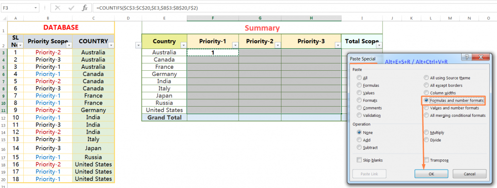
Figure 6: Formula is copied to the selected range using ‘Formulas and number formats’

Excel cell references in the formula perfectly address the criteria and make a dynamic formula (Figure 7).

Figure 7: Excel cell references make the dynamic formula

VI. HOW TO COPY A FORMULA WITHOUT ADJUSTING RELATIVE CELL REFERENCE

A. Method 1: Using the Formula Bar

If we need to copy the formula without any changes in the relative references, then follow these steps: 

(01) Select the cell that contains the formula we want to copy.

(02) Click inside the formula bar to activate Edit mode. 

(03) Use the mouse or keyboard to select the entire formula. 

(04) Copy the selected formula by Ctrl+C.

(05) Press the ‘Esc’ key to deactivate the formula bar. 

(06) Select the cell where we want a copy of the formula to appear. 

(07) Paste the formula by Ctrl+V. 

B. Method 2: Using the apostrophe (‘)

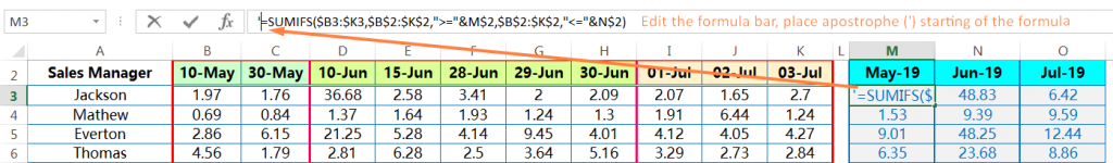
(01) Activate the formula bar and type an apostrophe (‘) at the beginning of the formula (that is, to the left of the equal sign) to convert it to text. 

(02) Press Enter to confirm the edit, copy the cell, and then paste it in the desired location. 

(03) After that, delete the apostrophe from both the source and destination cells to convert the text back to a formula. 

C. Method 3: Using the ‘Find and Replace’ Dialog Box (Ctrl+H) 

If the formulas placed in a number of ranges, then it is difficult to copy them to the other location one by one – either by using of formula bar; or by the use of the apostrophe. Then we use the third method – using the ‘Find and Replace’ dialog box. 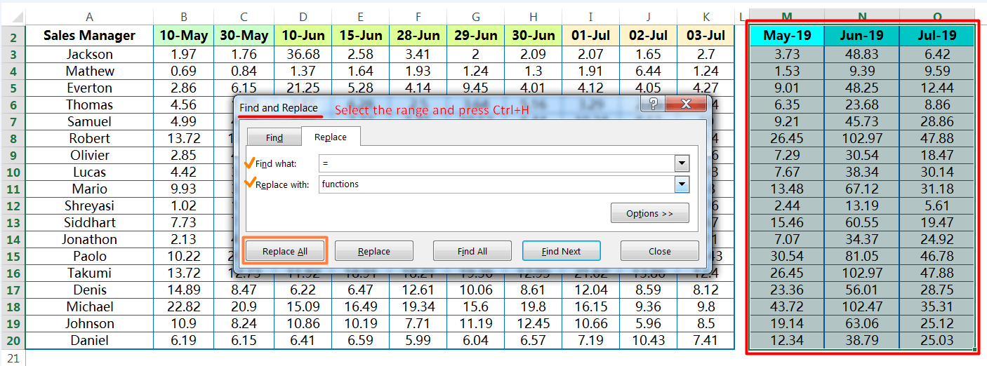 (01) Select the range with the formulas to want to copy.

(02) Press Ctrl+H to open the ‘Find and Replace’ dialog box.

(03)  Type equality sign (=) in front of the ‘Find what:’ box; and type any uncommon text, that does not relate to the topic, in front of the ‘Replace with:’ box.  For example, we use the text ‘functions’.

(04) Then press ‘Replace All‘.

(05) As a result, all the equality signs (=) have been replaced by the text ‘functions’. Now the formulas are converted to text. Copy the range and paste to the new locations.   

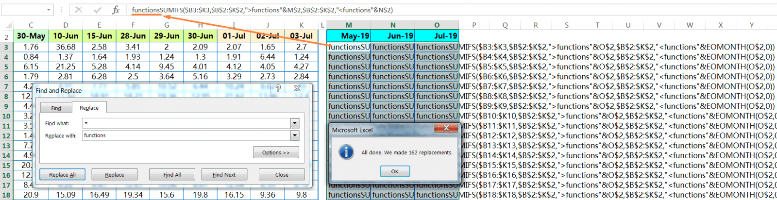
(06)  After the process is reversed. Press Ctrl+H to open the ‘Find and Replace’ dialog box. 

(07)  Type ‘functions’ in front of the ‘Find what:’ box; and type equality sign (=) in front of the ‘Replace with:’ box.  

(08) Then press ‘Replace All’.

■ Note: We had detail explained on Find and Replace in a separate tutorial. Request you read this tutorial: 07 Points Guided You How to Find And Replace in Excel?