
03 Best Ways: EXCEL DOUBLE VLOOKUP/ IFERROR VLOOKUP/ NESTED VLOOKUP

03 Best Ways: EXCEL DOUBLE VLOOKUP/ IFERROR VLOOKUP/ NESTED VLOOKUP
DOUBLE VLOOKUP is a term in Advance Excel where two VLOOKUP functions nested with the IFERROR function to make a nested formula that sequentially works in two different tables or columns of the same workbook or different workbooks and retrieves the value. Thus, Excel Double VLOOKUP is often known as IFERROR VLOOKUP or NESTED VLOOKUP.
Broadly, NESTED VLOOKUP is an advanced level of DOUBLE VLOOKUP where two or more VLOOKUP functions work together with two or more IFERROR functions, making a nested formula that sequentially works in two or more different tables or columns of the same workbook or different workbooks. NESTED VLOOKUP is a kind of IFERROR VLOOKUP in Excel.
The IFERROR function is a logic function that checks a cell to determine if that cell contains an error or if a formula will result in an error. If no error exists, the function returns the value of the formula. If an error exists, the function returns an error.
The IFERROR function can’t distinguish the type of error. The error could be #NAME, #N/A, #REF, DIV/0, and so on. What is used as the value_if_error argument will be displayed regardless of the error type.
A. SIMPLE METHOD OF DOUBLE VLOOKUP / IFERROR VLOOKUP / NESTED VLOOKUP
Excel Double VLOOKUP is a term where two VLOOKUP functions nested with the IFERROR function will make a unique formula, that is able to match the lookup_value in two different columns. It is also known as IFERROR VLOOKUP or NESTED VLOOKUP.
The logic behind the Excel DOUBLE VLOOKUP formula or IFERROR VLOOKUP formula is that when the first VLOOKUP fails to find the lookup_value in the first column range returns an Error, then the IFERROR function replaces the Error with the second VLOOKUP function which finds the same lookup_value in the second column range and retrieves the value.
As a result, with a single formula, we can retrieve the value matches with two different columns.
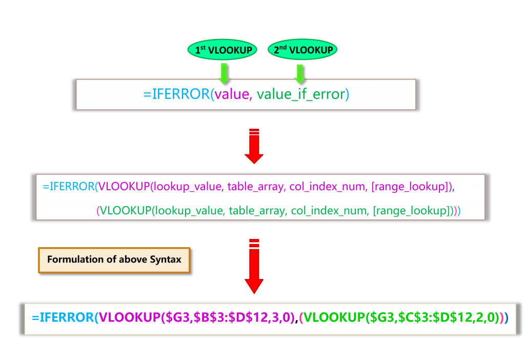
➢ SYNTAX:
➢ STEPS TO START:
=IFERROR(VLOOKUP($G3,$B$3:$D$12,3,0), (VLOOKUP($G3,$C$3:$D$12,2,0)))
• STEP 1: Select a cell to get the result of Double VLOOKUP (i.e., H3).
In this cell, place an equality “=” sign to start the formula and just type a few letters ‘=IF….‘ and select the IFERROR function from the Excel provided suggestion list with the help of a down arrow (↓) key, if required.

Then press the ‘Tab’ key, IFERROR syntax appears with the open parenthesis.

The IFERROR function has 2 arguments: value and value_if_error.
• Value is the expression being tested.
• Value_if_error is the text that will be returned if there is an error in the formula (or expression).
We place the first VLOOKUP in the value position and place the second VLOOKUP in the value_if_error position. Therefore, the new formula works in such a way, if the first VLOOKUP returns any #N/A error, it will be replaced by the value of the second VLOOKUP.
• STEP 2: Then type a few letters of vlookup such as ‘=vlo….’ and select the VLOOKUP function from the given suggestion list.

Then press the ‘Tab’ key, VLOOKUP syntax appears with the open parenthesis within the IFERROR function.

• STEP 3: The first VLOOKUP retrieves the value from a first table_array, likes
=IFERROR( VLOOKUP( $G3, $B$3:$D$12, 3, 0),
➢ $G3 – select the lookup value locates in cell G3 (i.e., CAN-1) and fix the Column address by pressing the F4 key thrice. Thus the range converts from the relative to the mixed cell reference where it indicates the absolute column and relative row.
As a result, while the formula is copied to the right side or horizontally, the column address does not change but the row address changes accordingly.
➢ $B$3:$D$12 – lookup_value found in the range is called lookup_array and fixed the range by pressing the F4 key once. Thus the range is converted to absolute from the relative cell reference.
As a result, the range does not change when the formula is copied to another cell either horizontally or vertically.
➢ 3 – the column_index_num is the count of columns between the lookup value column and the return value column.
➢ 0 – the last argument of the VLOOKUP function is range_lookup. If we are looking for an exact match, place either 0 or FALSE.
■ Note: We had detail explained on Cell Reference in a separate tutorial. Request you read this tutorial: 03 Types of Excel Cell Reference: Relative, Absolute & Mixed
• STEP 4: When the first VLOOKUP formula cannot find a match, it returns the #N/A error (i.e., lookup_value does not find a match in the first column of table_array).
Then the wrapped IFERROR function to replace the #N/A error either with the ‘values’ or ‘suggested texts’. We should place the texts in double quotation marks (” “).
But here the #N/A error is replaced with the values, those values are getting from the Second VLOOKUP.
We should place the second VLOOKUP in place of value_if_error, the second argument of the IFERROR function. Then, we write the formula as:
=IFERROR(VLOOKUP($G3, $B$3:$D$12, 3, 0), (VLOOKUP($G3, $C$3:$D$12, 2, 0)))
➢ $G3 – as the same as first Lookup, select the lookup value locates in cell G3 (i.e., CAN-1) and fix the Column address by pressing the F4 key thrice. Thus the range converts from the relative to the mixed cell reference where it indicates the absolute column and relative row.
As a result, while the formula is copied to the right side or horizontally, the column address does not change but the row address changes accordingly.
➢ $C$3:$D$12 – lookup_value found in the range is called lookup_array and in this case, lookup_array should be different from the first lookup_array.
Fixed the range by pressing the F4 key once. Thus the range is converted from the relative cell reference to the absolute.
As a result, the range does not change when the formula is copied to another cell either horizontally or vertically.
➢ 2 – the column_index_num is the count of columns between the lookup value column and the return value column.
➢ 0 – the last argument of the VLOOKUP function is range_lookup. If we are looking for an exact match we put either 0 or FALSE.
• STEP 5: Finally, press Enter to accept the formula. Formula ends by default and closes the last parenthesis as well.
• STEP 6: EXTEND THE FORMULA TILL THE END OF THE RANGE (WITHOUT FORMATTING)
Copy (Ctrl+C) the cell with formula ➪ Select the range of cells where to copy the formula (Shift+Down Arrow) ➪ Press either Alt+E+S+R (press sequentially, Alt, E, S, R) or Alt+Ctrl+V+R (press Alt+Ctrl+V, then R) which will select the “Formulas and number formats” in the Paste Special dialog box ➪ Then press Enter or click OK.

• STEP 7: OBSERVATIONS

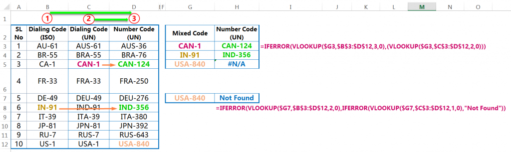
In the Excel double VLOOKUP two ranges are used for retrieving data: one is the range B3:D12 and the second one is C3:D12.
(01). In the first case, the lookup_value is CAN-1 and the Excel Double VLOOKUP returns the result value CAN-124 as a Number Code (UN). The lookup_value found in the range C3:D12.
(02). In the second case, the lookup_value is IN-91 and the Excel Double VLOOKUP returns the result value IND-356 as a Number Code (UN). The lookup_value found in the different range B3:D12.
(03). In the third case, the lookup_value is USA-840 and the Excel Double VLOOKUP returns the #N/A error. That means the lookup_value does not exist either in range C3:D12 or B3:D12.
(04). In the fourth case, using another IFERROR function to replace the #N/A error with a text likes “Not Found”. The text should be in double quotation. We can keep it blanks ” ” instead of a text.
B. ADVANCED METHOD OF DOUBLE VLOOKUP / IFERROR VLOOKUP / NESTED VLOOKUP
Nested VLOOKUP in Excel is an advanced level of multiple VLOOKUP functions in the IFERROR functions, where individual VLOOKUP function finds the match from the suggested table array and retrieves the value. If the VLOOKUP function fails to match, it returns a #N/A error.
The IFERROR function in Excel allows replacing the #N/A error with suggested ‘value’ or ‘text’. To make the formula more dynamic, rather than put any value manually replaces it with the second VLOOKUP. Similarly, the second VLOOKUP formula finds the match from another table array and retrieves the value. If it fails to find the match, it returns a #N/A error.
Again and again, apply the IFERROR function to replace the #N/A error by third, fourth, fifth,…returns by the VLOOKUP functions. The combination of multiple IFERROR and VLOOKUP functions makes a formula that allows to sequential lookup with first table array, second table array, third.., fourth…so on.
The advanced method of using the IFERROR VLOOKUP in Excel is called the Advanced Double VLOOKUP or Advanced Nested VLOOKUP or Advanced IFERROR VLOOKUP.
➢ SYNTAX:

➢ STEPS TO START:
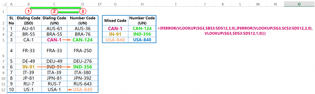
=IFERROR(VLOOKUP($G3,$B$3:$D$12,3,0), IFERROR(VLOOKUP($G3,$C$3:$D$12,2,0), VLOOKUP($G3,$D$3:$D$12,1,0)))
• STEP 1: Select the cell to get the result of Advanced Double VLOOKUP (i.e., H3).
In this cell, press equality “=” sign to start formula and just type a few letters of IFERROR e.g., =if…. and select the IFERROR function from the Excel provided suggestion list with the help of a down arrow (↓), if required.
Then press the ‘Tab’ key, IFERROR syntax appears with the open parenthesis.
The IFERROR function has two arguments: value and value_if_error.
We put the first VLOOKUP in place of the value argument and put the second VLOOKUP in place of the value_if_error argument. So, the new formula works in such a way, if the first VLOOKUP returns any #N/A error, it will be replaced by the value of the second VLOOKUP.
• STEP 2: Then type a few letters of the VLOOKUP, for example, =vlo… and select the VLOOKUP function from the Excel provided suggestion list.
Then press the ‘Tab’ key, VLOOKUP syntax appears with the open parenthesis within the IFERROR function.
• STEP 3: The first VLOOKUP retrieves the value from a first table_array. This formula allows retrieving the values against match cases and returns the #N/A errors in non-match cases.
In this case, we wrap the formula with another IFERROR function to replace the #N/A error. The #N/A error should be replaced with the value, this value comes from the Second VLOOKUP.
If the second VLOOKUP formula fails to find the match from the range, it returns the #N/A error. This error is replaced by the value of the third VLOOKUP.
The position of the first VLOOKUP in place of the ‘value’ argument of the first IFERROR function and in place of the ‘value_if_error’ argument puts the second IFERROR function. The position of the second VLOOKUP and third VLOOKUP in place of the ‘value’ and ‘value_if_error’ arguments in the second IFERROR function, respectively.
Therefore, now the formula works in such a way, if the first VLOOKUP returns any #N/A error, the second VLOOKUP replaces the error with the value. If the second VLOOKUP returns any #N/A error, it will be replaced by the value of the third VLOOKUP.
=IFERROR(VLOOKUP($G3,$B$3:$D$12,3,0), IFERROR(VLOOKUP($G3,$C$3:$D$12,2,0), VLOOKUP($G3,$D$3:$D$12,1,0)))
➢ $G3 – the lookup value locates in cell G3 (i.e., CAN-1) and same for the first, the second and the third VLOOKUP function.
Fix the Column address by pressing three times the F4 key. Thus the range converts from the relative to the mixed cell reference where it indicates the absolute column and relative row.
As a result, while the formula is copied to the right side or horizontally, the column address does not change but the row address changes accordingly.
➢ $B$3:$D$12 – lookup_array for the first VLOOKUP (lookup_array is the range where lookup_value is found).
$C$3:$D$12 – lookup_array for the second VLOOKUP.
$D$3:$D$12 – lookup_array for the third VLOOKUP.
Fixed every range by pressing the F4 key once. Thus the range is converted to absolute from the relative cell reference.
As a result, the range does not change when the formula is copied to another cell either horizontally or vertically.
➢ 3 – column_index_num for the first VLOOKUP (the column_index_num is the count of columns between the lookup value column and the return value column.
2 – column_index_num for the second VLOOKUP.
1 – column_index_num for the third VLOOKUP.
➢ 0 – the last argument of the VLOOKUP function is range_lookup. We are looking for an exact match, so we put either 0 or FALSE. So, range_lookup is the same for three VLOOKUP functions.
• STEP 4: Finally, press Enter to accept the formula. Formula ends by default and closes the last parenthesis as well.
• STEP 5: EXTEND THE FORMULA TILL THE END OF THE RANGE (WITHOUT FORMATTING)
Copy (Ctrl+C) the cell with formula ➪ Select the range of cells where to copy the formula (Shift+Down Arrow) ➪ Press either Alt+E+S+R (press sequentially, Alt, E, S, R) or Alt+Ctrl+V+R (press Alt+Ctrl+V, then R) which will select the “Formulas and number formats” in the Paste Special dialog box ➪ Then press Enter or click OK.
C. DYNAMIC METHOD OF DOUBLE VLOOKUP / IFERROR VLOOKUP / NESTED VLOOKUP
Using of MATCH function in the Advanced Double VLOOKUP (or Advanced Nested VLOOKUP or Advanced IFERROR VLOOKUP) makes it dynamic formula.
The MATCH() function returns the position of an item within an array that matches a specific value.
Using the MATCH() function in place of column_index_num automatically updates the column number that makes the dynamic formula.
The Syntax of the MATCH function is as follows:

➢ Lookup_value is the item to match. It can be a number, text string, a logical value, or a reference.
➢ Lookup_array is the table or an array containing all of the values to search.
➢ Match_type is a number that specifies how the match will be applied.
A match_type of zero (0) finds the first item in the array that is an exact match with the lookup_value.
To find the item closest to but less than the lookup_value, use a match_type of -1.
To find the item closest to but greater than the lookup_value, use a match_type of 1.
In the last two cases, the values in the lookup_array must be in ascending order for the MATCH function to work correctly.
The match_type is optional and will default to 1 if omitted from the arguments
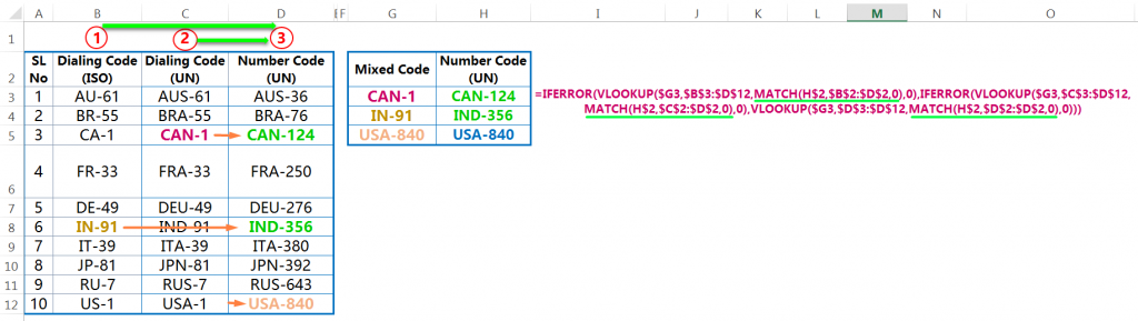
➢ SYNTAX:

➢ STEPS TO START:
• STEP 1: Select the cell to get the result of Advanced Double VLOOKUP (i.e., H3).
In this cell, press equality “=” sign to start formula and just type a few letters of IFERROR e.g., =if…. and select the IFERROR function from the Excel provided suggestion list with the help of a down arrow (↓), if required.
Then press the ‘Tab’ key, the IFERROR syntax appears with the open parenthesis.
The IFERROR function has two arguments: value and value_if_error.
We put the first VLOOKUP in place of the value argument and put the second VLOOKUP in place of the value_if_error argument. So, the new formula works in such a way, if the first VLOOKUP returns any #N/A error, it will be replaced by the value of the second VLOOKUP.
• STEP 2: Then type a few letters of the VLOOKUP, for example, =vlo… and select the VLOOKUP function from the Excel provided suggestion list.
Then press the ‘Tab’ key, VLOOKUP syntax appears with the open parenthesis within the IFERROR function.
• STEP 3: The position of the first VLOOKUP in place of the ‘value’ argument of the first IFERROR function and in place of the ‘value_if_error‘ argument puts the second IFERROR function. The position of the second VLOOKUP and third VLOOKUP in place of the ‘value‘ and ‘value_if_error‘ arguments in the second IFERROR function, respectively.
So, the formula works in such a way, if the first VLOOKUP returns any #N/A error, the second VLOOKUP replaces the error with the value. If the second VLOOKUP returns any #N/A error, it will be replaced by the value of the third VLOOKUP.
=IFERROR(VLOOKUP($G3,$B$3:$D$12, MATCH(H$2,$B$2:$D$2,0),0),
IFERROR(VLOOKUP($G3,$C$3:$D$12, MATCH(H$2,$C$2:$D$2,0),0),
VLOOKUP($G3,$D$3:$D$12, MATCH(H$2,$D$2:$D$2,0),0)))
➢ EXPLANATION OF THE FIRST VLOOKUP FUNCTION:
VLOOKUP($G3,$B$3:$D$12, MATCH(H$2,$B$2:$D$2,0),0)
• $G3 – the lookup value locates in cell G3 (i.e., CAN-1) and the same for the first, the second and the third VLOOKUP function.
Fix the Column address by pressing the F4 key thrice. Thus the range converts from the relative to the mixed cell reference where it indicates the absolute column and relative row.
As a result, while the formula is copied to the right side or horizontally, the column address does not change but the row address changes accordingly.
• $B$3:$D$12 – lookup_array for the first VLOOKUP (lookup_array is the range where lookup_value is found).
• MATCH(H$2,$B$2:$D$2,0) – we place the MATCH() function in place of column_index_num to update the column number automatically. Please note that the lookup column in both the lookup_array of the VLOOKUP function and the lookup_array of the MATCH function should be the same. Otherwise, the formula returns the #N/A error. In both cases, Column B is the lookup column.
- H$2 = lookup_value reference to ‘Number Code (UN)’ and fixed the row address by pressing two times F4 Key. As a result, the lookup_value is converted from the relative cell reference to the mixed column cell reference, where it indicates the relative column and absolute row address.
As a result, while the formula is copied to the other cells, the row address does not change but the column address changes accordingly.
- $B$2:$D$2 = lookup_value found in the range is called lookup_array and fixed the range by pressing a single time F4 key. Thus the range is converted from the relative cell reference to the absolute cell reference.
As a result, the range does not change when the formula is copied to another cell either horizontally or vertically.
- 0 = for exact match
• 0 – range_lookup, the last argument of VLOOKUP function. The value zero (0) or FALSE signifies the exact match.
➢ EXPLANATION OF THE SECOND VLOOKUP FUNCTION:
VLOOKUP($G3, $C$3:$D$12, MATCH(H$2,$C$2:$D$2,0), 0)
We should follow the same steps described in the first VLOOKUP function.
➢ EXPLANATION OF THE THIRD VLOOKUP FUNCTION:
VLOOKUP($G3,$D$3:$D$12, MATCH(H$2,$D$2:$D$2,0),0)
We should follow the same steps described in the first VLOOKUP function.
• STEP 4: Finally, press Enter to accept the formula. Formula ends by default and closes the last parenthesis as well.
• STEP 5: EXTEND THE FORMULA TILL THE END OF THE RANGE (WITHOUT FORMATTING)
Copy (Ctrl+C) the cell with formula ➪ Select the range of cells where to copy the formula (Shift+Down Arrow) ➪ Press either Alt+E+S+R (press sequentially, Alt, E, S, R) or Alt+Ctrl+V+R (press Alt+Ctrl+V, then R) which will select the “Formulas and number formats” in the Paste Special dialog box ➪ Then press Enter or click OK.
D. CONCLUSION
(01). Excel Double VLOOKUP (or IFERROR VLOOKUP or Nested VLOOKUP) is the most important formulas in Advance Excel. The formula helps to reduce the time span in data analysis.
(02). Multiple VLOOKUPS nested with IFERROR function make an advanced formula in Advance Excel that works sequentially in two or more tables or columns in the same workbook or the different workbooks.
(03). Using of MATCH function in Advanced Double VLOOKUP (or Advanced Nested VLOOKUP or Advanced IFERROR VLOOKUP) makes it a dynamic formula.


Leave a Comment