29 ways to save time with Excel formulas

29 ways to save time with Excel formulas

Formulas are the bread and butter of Excel. If you use Excel on a regular basis, I bet you use a lot of formulas. But crafting a working formula can take way too much time. In this article, I share some good tips to save you time when working with formulas in Excel.

1. Don't add the final parentheses to a function

Let's start out with something really easy! When you entering one function on it's own (SUM,AVERAGE, etc.) you don't need to enter the final closing parentheses. For example, you can just enter:

=SUM(A1:A10

and press return. Excel will add the closing parentheses for you. It's a small thing, but convenient.

Note: this won't work if your formula contains more than one set of parentheses.

2. Move a formula and keep references from changing

One of Excel's most powerful features is relative addresses — when you copy a formula to a new location all relative addresses will change. Often this is exactly what you want, because the reuse of formulas is one of the most important techniques of a well-built, easy to maintain worksheet.

But sometimes you need to move or copy a formula to a new location and you don't want the formula to change at all. There several ways you can do this.

If you're just moving a formula to a nearby location, try drag and drop. Dragging will keep all addresses intact and unchanged.

If you moving a formula to a more distant location, use cut and paste. (Win: Ctrl + X, Ctrl + V  Mac:  Cmd + X, Cmd + V )  When you cut a formula, it's references do not change.

3. Copy a formula and keep references from changing

Note: you could change all cell references to make them absolute, but this tip assumes that you don't want to do that, for whatever reason.

If you just need to copy a single formula, select the entire formula in the formula bar and copy to the clipboard. You can then paste at a new location. The result will be a formula identical to the original.

To copy a group of formulas to a new location without affecting references, you can use find and replace. Select the formulas you want to copy, then search for and replace the equal (=) sign in the formulas with the hash (#)  character. This will convert the formulas to text. Now copy and paste the formulas to a new location. After you paste the formulas, and with all formulas selected, reverse the search and replace process. Search for the hash (#) and replace an equal sign (=). This will restore the formulas to working order. (Credit: Tom Urtis)

4. Double click the fill handle to copy down formulas

When you're adding formulas to tables, one of the things you do most often is copy the formula from the first row of the table to the last row of the table. If you know the keyboard shortcuts for navigating data in Excel, you can use them to quickly paste in a whole column of formulas in just a few key strokes. However, the fill handle is even faster, because there's no need to navigate to the bottom of the table.

The fill handle is the little rectangle that sits in the lower right corner of all selections in Excel. As long as the formula sits in a column next to another column will a full set of data, you can just double-click the fill handle to copy the formula all the way down to the bottom of the table.

Note: This tip won't work if there's not a full column of data the left of the formula you are entering. Excel uses this data to figure out how far down the worksheet to copy the formula. You can use this next approach however...

If the selection is not too large, you can also fill formulas down a worksheet using the shortcut for Fill Down (Control + D). Just make sure to select the original formula and the target cells first. This is faster than copy/paste, but not as fast as the fill handle, especially if you are copying the formula into a large group of cells.

Video: Shortcuts to move around a big list fast

5. Use a table to enter formulas automatically

An even faster way to enter formulas is to first convert your table to an official Excel Table. The terminology here is confusing, since any data with more than one column is technically a "table" but Excel has a formal structure called a Table that provides many benefits. Once you convert your data to a table (Both platforms: Ctrl + T), all formulas you enter in the first row will be automatically copied down the full length of the table. This saves a lot of time and also helps to prevent errors.

As a bonus, when ever you update a formula in a table, Excel will again update all like formulas in the same column.

Note: formulas in a table will automatically use structured references (i.e. in the example above =[@Hours]*[@Rate] instead of =C4*D4. However, you can type cell addresses directly and they will be preserved.

6. Use AutoComplete + tab to enter functions

When you enter an equal sign and start typing, Excel will start matching the text you enter against the huge list of functions that are available. As you type, you'll see a list of "candidate" functions appear below. This list will narrow with each letter you type. Once the function you want is selected in the list, you can "ask" Excel to enter it for you by pressing tab. On Windows, functions are selected automatically as you type. On a Mac options are presented but not selected, so you need to take one more step: use the arrow key to select the function you want, then press tab or return to have Excel enter the function for you.

7. Use Control + click to enter arguments

Don't like typing commas between arguments? You can have Excel will do it for you. When you're entering arguments in a function, just hold down Control (Mac: Command) as you click each reference and Excel will automatically enter commas for you. For example, you can enter a formula like: =SUM(A1, B10, C5:C10) by entering "=SUM(" then Control-clicking each reference. This will work with any function where you are supplying references as arguments.

8. Use the formula tip window to select arguments

Whenever you're working with a formula that contains an Excel function, remember that you can always use the hint window to select arguments. This can be real time-saver if the formula is complicated, especially if it contains lots of nested parentheses. To select arguments, work in two steps. In step one, click to put the cursor inside the function whose argument you want to select. Excel will then display a hint for that function that shows all arguments. In step two, click the argument you want to select. Excel will select the entire argument, even when it contains other functions or formulas. These is a nice way to select arguments when using F9 to debug a formula.

Want to learn more? We offer an entire course on Excel formulas and functions.

9. Insert function argument placeholders with a shortcut

Normally, as you enter a function, Excel will present tips about each arguments as you add commas. But sometimes you might want to have Excel add placeholders for all the function arguments at once. If so, you'll be glad to know that there's a shortcut for that.

When you're entering a function, after Excel has recognized the function name, type Control + Shift + A (both platforms). For example, if you type "=DATE(" and then use Control + Shift + A, Excel will give you "=DATE(year,month,day)". You can then double-click each argument (or use the Function tip window to select each argument) and change it to the value you want.

10. Move the "formula thing" out of your way

Sometimes when you're entering a formula, the formula hint window gets in your way, blocking your view of other cells you want to see on the worksheet. When that happens, remember that you can move the hint window out of your way. Just mouse over the edge of the window until you see the cursor change, then click and drag to a new location. Then you can continue entering or editing your formula. Depending on the structure of your worksheet, another way to manage this problem is to edit the formula in the formula bar instead of directly in the cell.

11. Toggle the display all formulas at once

Whenever you edit a cell that contains a formula, Excel automatically displays the formula instead of it's result. But sometimes you might way to see all of the formulas on a worksheet at one time. To do this, just use the keyboard shortcut for displaying formulas: Control + ~ (that's a tilde). With this shortcut, you can rapidly toggle the display all formulas on a worksheet or off. This is a nice way to see all formulas at once, and to check formulas for consistency.

12. Select all formulas in a worksheet at once

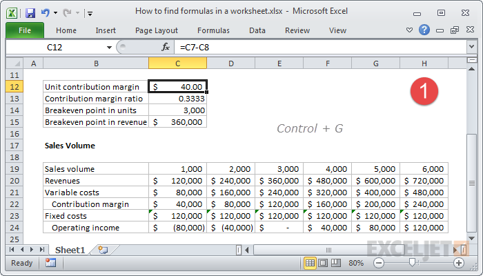
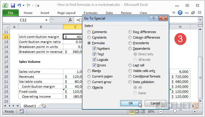
Another way to see all formulas in a worksheet is to select them. You can do this using of the more powerful (and hidden) features in Excel: is Go To > Special (Ctrl + G). With this command, you can select all sorts of interesting things in Excel, including blank cells, cells that contain numbers, cells that are blank, and much more. One of the options is cells that contain formulas. To select all cells that contain formulas on a worksheet, just type Ctrl + G to bring up the Go To dialog box, then click the Special button, then select Formulas. When you click OK, all cells that contain formulas will be selected.

If you want to select only a subset of formulas in a worksheet, make a selection first, then use the same command.

13. Use paste special to convert formulas to static values

A common problem in Excel is a need to stop calculated values from changing. For example, maybe you want to simplify a worksheet by removing "helper" columns that you used to generate certain values. But if you delete these columns with formulas still referring to them, you'll get a load of #REF errors. The solution is to first convert formulas to values, then delete the extra columns. The simplest way to do that is to to use Paste Special. First, select the formulas you want to convert and Copy to the clipboard. Next, with the formulas still selected, open the Paste Special dialog (Win: Ctrl + Alt + V, Mac: Ctrl + Cmd + V) and use the Values option. This will replace all formulas you selected with the values they had calculated.

14. Use Paste Special to adjust values in place

Another common problem in Excel is a need to change a lot of values in place. For example, perhaps you have a list of 500 product prices and you need to increase all prices by 5%. Or maybe you have a list of 100 dates that all need to be moved into the future by one week? In such cases, you could add a "helper" column to your table, perform the required calculation, convert the results to values, then copy them over the original column. But if you only need a simple calculation, Paste Special is much simpler and faster, because you can change the value directly without any extra formulas.

For example, to convert a set of dates in place to one week later, do this: add the number 7 to any cell in the worksheet, then copy it to the clipboard. Next, select all of the dates you want to change. Then, use Paste Special > Operations > Add. When you click OK, Excel will add the number 7 to the dates you've selected, moving them forward in time by 7 days, with no need to create helper columns.

To increase a set of prices by 10%, use the same approach. Enter 1.10 into a cell, and copy it to the clipboard. Then select the prices you want to change, and use Paste Special > Operations > Multiply to convert all prices in place. Once you get the hang of this tip, you'll find lots of clever uses for it.

Note: this only works with values. Don't try it with formulas!

15. Use named ranges to make formulas more readable

One of the oldest pro tips in the book is to use named ranges in your formulas to make them more readable. For example, let's say you have a simple worksheet that shows hours worked for a small team. For each person, you want to multiply their hours worked times a single hourly rate. Assuming the hourly rate is in cell A1, your formulas might look like this:

=B3 * $A$1
=B4 * $A$1
=B5 * $A$1

But if you name cell A1 "hourly_rate", your formulas will look like this:

=B3 * hourly_rate
=B4 * hourly_rate
=B5 * hourly_rate

Naming ranges this way makes formulas a lot more readable, and saves entering a lot of dollar signs ($) to create absolute references.

Naming ranges is easy. Just select the range/cell(s) you want to name, then type a name in the namebox and press enter. Now that you've named a range, Excel will use it whenever you point and click on the range as you're building a formula — when you click a named range, you'll see it's name automatically inserted into the formula. As a bonus, you can also easily navigate to the named range whenever you like. Just select the name from the drop-down that appears next to the name box.

16. Apply names to existing formulas automatically

What happens when you've already created formulas and then create a named range you want to use in them? Nothing, actually. Excel won't make any changes to your existing formulas or offer to apply the new range names automatically. However, there is a way to apply range names to existing formulas. Just select the formulas you want to apply names to, then use the Apply Names feature.

Once the Apply Names window is open, select the names you want to apply and click OK. Excel will replace any corresponding references with the names you selected.

17. Save a formula that's not done

If you're working with a more complex formula, there's a good chance it will take a while to get the formula working right.  But you might be short on time and need to come back to the formula later to get it working like you want. Unfortunately, Excel won't let you enter a formula that's broken. If you try, Excel will complain loudly that the formula has errors, and won't let you continue until you've resolved all problems.

However, there's an easy workaround: just temporarily convert the formula to text. To do this, you can either add a single apostrophe to the start of the formula (before the =), or just remove the equal sign altogether. In both cases, Excel will stop trying to evaluate the formula and will let you enter it as-is. Later, you can come back to the formula and resume work.

18. Be aware of the functions that Excel offers

Functions exist to solve specific problems. You can think of a function as a pre-built formula with a specific name, purpose, and return value. For example the PROPER function has just one purpose: it capitalizes words. Give it text like "nEW york CiTY", and it will give you back "New York City". Functions are incredibly handy when they solve a problem that you have, so it make sense to familiarize yourself with the functions available in Excel.

See: Excel Function Guide and 500 Excel Formula Examples for a list of commonly used functions and formulas that use them.

Note: People are often confused by the terminology used to talk about functions and formulas. An easy way to think about it is this: everything that starts with an equal sign in Excel is a formula. By this definition, all functions are formulas too, and formulas can contain multiple functions.

19. Use F4 to toggle relative and absolute references

The key to constructing formulas that you can be elegantly copied to new locations and still work correctly, is using the right combination of absolute and relative references. The reason this is so important is because it allows you to reuse existing formulas instead of creating new ones, and reusing the same formula drastically reduces the possibility of errors in a workbook by limiting the number of formulas that need to be checked.

However, converting references back and forth between relative and absolute references can be a nuisance — typing in all those dollar signs ($) is tedious and error-prone. Luckily, there's a great shortcut that allows you to quickly toggle through the 4 options available for each reference: (Windows: F4, Mac: Command + T). Simply put the cursor into a reference use the shortcut. Each time you use it, Excel will "rotate" to the next option in this order: fully relative (A1) > fully absolute ($A$1) > Absolute row (A$1) > absolute column ($A1).

20. Remember that formulas and functions return a value. Always.

When you're struggling with a formula, sometimes it's because you think part of the formula is returning a certain value but it fact it is returning something else. To check what is actually being returned by a function or by part of a formula, use the F9 tip below.

Note: The word "return" comes from the world of programing, and it sometimes confuses people new to this concept. In the context of Excel formulas, it's used like this "The LEN function returns a number" or "The formula in cell A1 returns an error". Whenever you hear the word "return" with formula, just think "result".

21. Use F9 to evaluate parts of a formula

The shortcut F9 (fn + F9 on a Mac) can solve parts of a formula in real time. This is a fantastic tool for debugging larger formulas, when you need to verify that the result of a particular part of the formula is what you're expecting. To use this tip, edit the formula and select the expression or function you want to evaluate (tip - use the function tip window to select entire arguments). One you have a selection, press F9. You'll see that part of the formula replaced by the value it returns.

Note: On Windows, you can undo F9, but this doesn't seem to work on a Mac. To exit the formula without making changes, just use Esc.

Video: How to check and debug a formula with F9

22. Use Formula Evaluator to solve a formula step by step

When using F9 to evaluate a formula becomes too tedious, it's time to break out bigger hardware: Evaluate Formula. Evaluate Formula solves a formula one step at a time. Each time you click the Evaluate button, Excel will solve the underlined part of the formula and show you the result. You can find Evaluate Formula on the Formulas tab of the ribbon, in the Formula Auditing group. To use Evaluate Formula, select a formula, and click the button on the ribbon.  When the window opens, you'll see the formula displayed in a text box with an Evaluate button below. One part of the formula will be underlined — this is the part currently "under evaluation". When you click evaluate, the underlined portion of the formula is replaced with the value it returns. You can keep clicking evaluate until the formula is fully solved.

Video: How to Evaluate Complex Formulas

Note: Evaluate formula is only available in the Windows version of Excel. The Mac version takes a different approach, called Formula Builder, which displays results as you create a formula. It's not quite the same functionality, but it is very helpful, and you can use it with formulas that already exist.

23. Build complex formulas in small steps

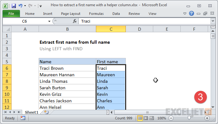
When you need to build a more complex formula, and aren't sure how to do it, start with the general approach and some hard-coded values. Then add in more logic to replace the hard-coded values one step at a time. For example, let's say you want to write a formula that extracts the first name from a full name. You know you could use the LEFT function, to pull text from the left, but you're not sure how to calculate the the number of characters to extract. Start with   LEFT(full_name, 5) to get the formula working. Then figure out how to to replace the number 5 with a calculated value. In this case, you can work out the number of characters to extract by using the FIND function to locate the position of the first space character.

Video: How to build a complex formula step by step

24. Use named ranges like variables

In many cases, it makes sense to use named ranges like variables to make your formulas more flexible and easier to work with. For example, if you're doing a lot of concatenation (joining text values together), you may want to create your own named ranges for new line characters, tab characters, etc. This way, you can simply refer to the named ranges directly instead of adding a lot of complex syntax to your formulas. As a bonus, if your named ranges contain text values,  you don't need to use any quotation marks around the text when you add them to a formula. This idea a little hard to explain so see this video for a detailed example.

25. Use concatenation in labels to make assumptions clear

When you create a worksheet that relies on certain assumptions, it can be a challenge to clearly show the assumptions you're making. Often, you'll have a certain area on the worksheet for inputs and another area for outputs, and there isn't room to show both at the same time. One way to make sure key assumptions are clear is to embed them directly into labels that appear on the worksheet using concatenation, usually with the TEXT function.

For example, normally, you might have a label that says "Coffee cost" followed by a calculated cost. With concatenation, you can make the label say "Coffee cost ($2.00/cup): which makes it clear that you have assumed a cost of $2.00/cup.

Video: clarify assumptions with concatenation

26. Add line breaks to nested IFs to make them easier to read

When you're creating a nested IF formula, keeping track of true and false arguments in a blizzard of parentheses can get very confusing. As you wrangle the parentheses, its easy to make a mistake in the logic. However, there is a simple way make a formula with multiple IF statements much easier to read: just add line breaks to the formula after each TRUE argument. This will make the formula read more like a table.

Video: How to make nested IFs easier to read

27. Enter functions with AutoComplete

When you're entering a function, excel will try to guess the name of the function you want, and present an AutoComplete list for you to select from. The question is, how do you accept one of the options displayed and yet still stay in edit mode? The trick is to use the tab key. When you press tab, Excel adds the complete function and leaves the cursor active in the parentheses so that you can fill in the arguments as needed. On a Mac, you need to use the down arrow key first to select the function you want to add, then press Tab to insert the function.

28. Use AutoSum to enter SUM formulas

You don't always get the chance to use this AutoSum, but when you do, it's satisfying. AutoSum works for both rows and columns. Just select an empty cell to the right or below the cells you want to sum, and type Alt + = (Mac: Command + Shift + T). Excel will guess the range you are trying to sum and insert the SUM function in one step. If you want to be more specific, so that Excel doesn't guess, first select the range you intend to sum, including the cell where you'd like the SUM function to be.

AutoSum will even insert multiple SUM functions at the same time. To sum multiple columns, select a range of empty cells below the columns. To sum multiple rows, select a range of empty cells in a column to the right of the rows.

Finally, you can use AutoSum to add both row and column totals at the same time for an entire table. Just select a full table of numbers, including empty cells below the table and to the right of the table, and use the shortcut. Excel will add the appropriate SUM functions in the empty cells, giving you column totals, row totals, and a grand total in a single step.

29. Enter the same formula in multiple cells at once

Often, you'll need to enter the same formula into a group of cells. You can actually do this in one step with the keyboard shortcut Control + Enter. Just select all the cells at the same time, then enter the formula normally as you would for the first cell. Then, when you're done, instead of pressing Enter, press Control + Enter. Excel will add the same formula to all cells in the selection, adjusting references as needed. When you use this approach you don't have to copy and paste, fill down, or use the fill handle. You're done in one step.

You can also use this same technique to edit multiple formulas at the same time. Just select all of the formulas at once, make the change you need, and press Control + Enter.