
How to Use XLOOKUP for Reverse Order Search
How to Use XLOOKUP for Reverse Order Search
Bottom Line: Learn how to use XLOOKUP to search in reverse order from bottom to top (last-to-first) to return the last date.
Skill Level: Intermediate
Download the Excel File
The file that I work within the video can be found below. You can also download the “Follow Along” version if you'd like to practice building out the report.
Compatibility: This file uses the new Dynamic Array Functions that are only available on the latest version of Office 365. This includes both the desktop and web app versions of Excel.
I'm planning to post a bonus episode in this series that covers how to make the dashboard with older versions of Excel using pivot tables instead.
Building an Attendance Dashboard
This post is part 2 of a six-part series explaining how to build an interactive dashboard for attendance. This attendance report was an entry for the Excel Hash competition. I recommend you check out the first post here:
Using XLOOKUP
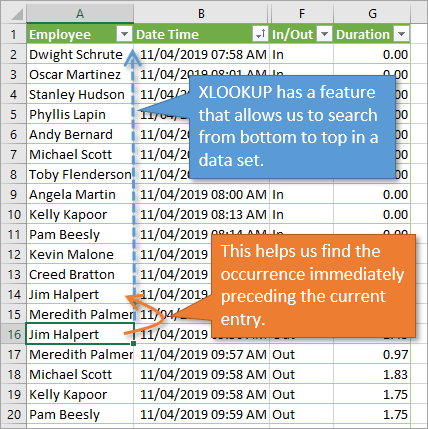
In the first part, we determined which entries are “In” and which are “Out,” using the XOR function. Now we need to determine how long each employee was in the building so we can calculate their total time at work.
To do this, we are going to utilize a helpful new function called XLOOKUP (article & video on XLOOKUP). Among other great abilities, this function can help us to search a set of entries from in reverse order, from last to first. This feature is helpful because for any “out” entry, we can find the “in” entry that was directly before it, and then calculate the duration between them.
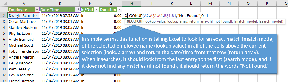
The XLOOKUP function has six arguments. The last 3 are optional but used in this scenario:
- Lookup Value: This is what you want the function to search for. For our example, we are looking for an employee's name.
- Lookup Array: This is the range that you want it to search in. In our case, we want to search for everything above the current cell (see running total reference section below).
- Return Array: The range that you want to return a value from. For our report, we want to return the date/time entry.
- If Not Found: The value to return if the lookup value is not found in the lookup array. I just used “Not Found” but you could choose any word or value, including a blank. We can use this in place of wrapping the function in IFERROR.
- Match Mode: Allows you to specify an exact or approximate match. I chose the “Exact match” to find the exact employee name, represented by 0.
- Search Mode: Allows you to search in regular or reverse order. In our case, we want to search last-to-first, represented by -1.
Running Total References
For the lookup and return arrays we are using a running total reference. This is a mixed absolute/relative reference that refers to all the cells at and above the row the formula is in.
If the formula is in row 7, the range reference will look like the following.
A$1:A7
The starting row will always be anchored at row 1. This allows to always perform the search above the current row to find the previous occurrence of the employee's name.
When all is said and done, our XLOOKUP function in Row 2 of our spreadsheet looks like this:
=XLOOKUP(A2,A$1:A1,B$1:B1,”Not Found”,0,-1)
Calculating the Duration
Once we have plugged in the XLOOKUP values, we can calculate the duration. This is just a simple formula that subtracts the previous timestamp from the current timestamp. The result will most likely be formatted as a decimal indicating a fraction of the day. If so, just multiply that result by 24 hours.
Now, we only want to calculate duration on the “Out” entries (subtracting the time the employee arrived from the time the employee left). If we subtracted their out time from their in time, we would be calculating the duration of time they spent away from the office, which is not what we are looking for.
To make sure that we're only dealing with time spent at work, we can just wrap our existing formula in an If Statement:
If the value in the In/Out column is “Out” then return the answer, and if not, return a zero.
Running Totals with Structured References
As I described in my previous post, using normal references can sometimes lead to errors when new entries are added to your Tabel. To avoid this, you can build the same formula using the INDEX function and structured (table) references.
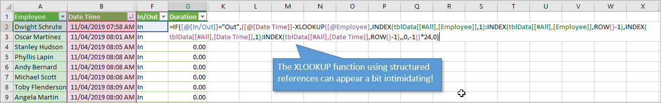
The following formula is used for the lookup array in XLOOKUP.
INDEX(tblData[[#All],[Employee]],1):INDEX(tblData[[#All],[Employee]],ROW()-1)
This formula creates a reference from the header row to the cell ABOVE the row that the formula is in. It uses the INDEX function and the ROW function to create a reference to the cell above.
The final formula looks long and scary but isn't too bad once you break it down into pieces. The color-coding in the image below might help you to better break it down.
I walk you through these structured references in more detail in the video.
Conclusion
In the next video, we will use these duration totals that we calculated to analyze employee attendance. We'll be able to break down attendance hours for individuals as well as departments.


Leave a Comment