
How to Use Index Match Instead of Vlookup
How to Use Index Match Instead of Vlookup
Bottom Line: Learn how to use the INDEX and MATCH functions as an alternative to VLOOKUP.
Skill Level: Beginner
Download the Excel File
Here is the Excel file that I used in the video. I encourage you to follow along and practice writing the formulas.
Advantages of Using INDEX MATCH instead of VLOOKUP
It's best to first understand why we might want to learn this new formula. There are two main advantages that INDEX MATCH have over VLOOKUP.
#1 – Lookup to the Left
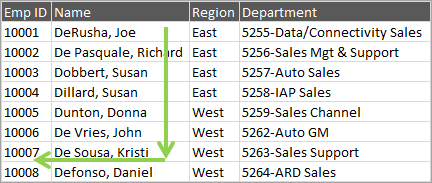
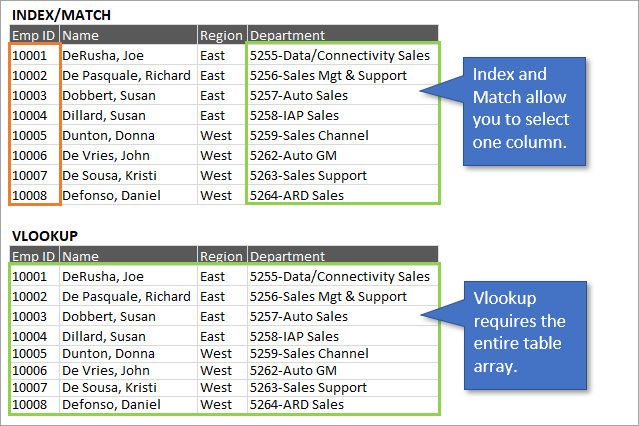
The first advantage of using these functions is that INDEX MATCH allows you to return a value in a column to the left. With VLOOKUP you're stuck returning a value from a column to the right.
Yes, you can technically use the CHOOSE function with VLOOKUP to lookup to the left, but I wouldn't recommend it (performance test).
#2 – Separate Lookup and Return Columns
Another benefit is that you specify a single column for both the lookup and return ranges, instead of the entire table array that VLOOKUP requires.
Why is this a benefit? Because VLOOKUP formulas tend to break when columns in a table array get inserted or deleted. The calculation can also slow down if there are other formulas or dependencies in the table array.
With INDEX MATCH there's less maintenance required for your formulas when changes are made to your worksheet.
Wrapping Your Head Around INDEX MATCH
An INDEX MATCH formula uses both the INDEX and MATCH functions. It can look like the following formula.
=INDEX($B$2:$B$8,MATCH(A12,$D$2:$D$8,0))
This can look complex and overwhelming when you first see it!
To understand how the formula works, we'll start from the inside and learn the MATCH function first. Then I'll explain how INDEX works. Finally, we will combine the two in one formula.
The MATCH Function is Similar to VLOOKUP
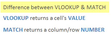
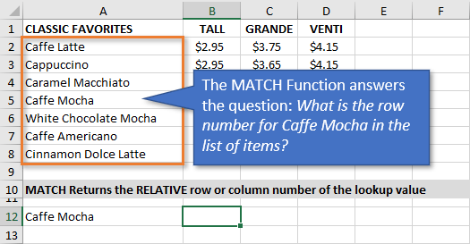
The MATCH function is really like VLOOKUP's twin sister (or brother). Its job is to look through a range of cells and find a match. The difference is that it returns a row or column number, NOT the value of a cell.
The following image shows the Excel definition of the MATCH function, and then my simple definition. This simple definition just makes it easier for me to remember the three arguments.
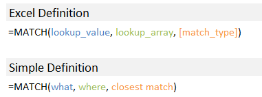
The MATCH function's arguments are also similar to VLOOKUP's. MATCH's lookup_array argument is a single row/column. Therefore, we don't need the column index number argument that VLOOKUP requires.
=MATCH(lookup_value, lookup_array, [match_type])
=VLOOKUP(lookup_value, table_array, col_index_number, [range_lookup])
Let's dive into an example to see how MATCH works.
An Example of the Match Function
We'll use my Starbucks menu example to learn MATCH. In this case, we want to use the MATCH function to return the row number for “Caffe Mocha” from the list of items in column A.
Here are instructions on how to write the MATCH formula.
1. lookup_value – The “what” argument
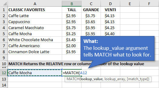
In the first argument, we tell MATCH what we are looking for. In this example, we are looking for “Caffe Mocha” in column A. I have entered the text “Caffe Mocha” in cell A12 and referenced the cell in the formula.
2. lookup_array – The “where” argument.
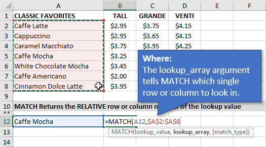
Next, we need to tell MATCH where to look for the lookup value. I selected the range $A$2:$A$8, which contains the list of items. MATCH will look through this column from top-to-bottom until it finds a match.
I made this an absolute reference (F4 on the keyboard) so that the range does not change if we copy the formula down. It's good to get in the habit of doing this after selecting the lookup_array range.
Note: You can also specify a row for this argument. In that case, MATCH would look across the column from left-to-right to find a match.
3. [match_type] – The “closest/exact” match argument
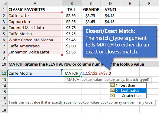
Here we specify if the function should look for an exact MATCH, or a value that is less than or greater than the lookup_value.
MATCH defaults to 1 – Less than. So we always need to specify a 0 (zero) for an exact match. This is similar to specifying FALSE or 0 (zero) for the last argument in VLOOKUP.
When your MATCH is looking up text you will generally want to look for an exact match.
If you are looking up numbers with the MATCH function then the “Less than” or “Greater than” match types can be very useful for tax and commission rate calculations.
The Result
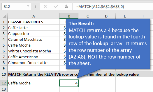
The MATCH function returns a 4. This is because it finds the lookup value in the 4th row of the lookup_array (A2:A8).
It's important to note that this is NOT the row number of the sheet. The row/column number that MATCH returns is relative to the lookup_array (range).
Now that we have a basic understanding of how MATCH works, let's see how INDEX fits in.
The Index Function
The INDEX function is like a roadmap for the spreadsheet. It returns the value of a cell in a range based on the row and/or column number you provide it.
There are three arguments to the INDEX function.
=INDEX(array, row_num, [column_num])
The third argument [column_num] is optional, and not needed for the VLOOKUP replacement formula.
So, let’s look at the Starbucks menu again and answer the following question using the INDEX function.
“What is the price of the Caffe Mocha, size Grande?”
1. array – The “where” argument.
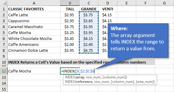
This argument tells the INDEX where to look in the spreadsheet. I specified $C:$2:$C$8 because this range is the column of prices that I want to return a value from.
Again, it's good practice to make this range an absolute reference so you can copy the formula down.
2. row_num – The “row number” argument
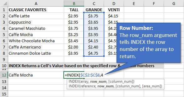
Next, we specify the row number of the value we want to return within the array (range). This is the row number of the array, NOT the row number of the sheet.
For now, we can hard code this number by typing a 4 into the formula.
The Result
The result is $3.95, the value in the 4th cell of the array (range).
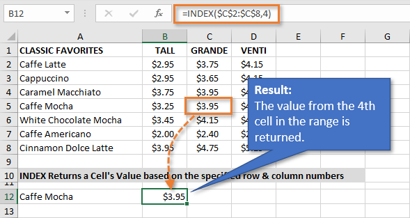
Important Note: The number formatting from the array range does not automatically get applied to the cell that contains the formula. If you see a 4 returned by INDEX, this means you need to apply a number format with decimal places to the cell(s) with the formula.
INDEX is pretty simple on its own. Let's see how to combine it with MATCH.
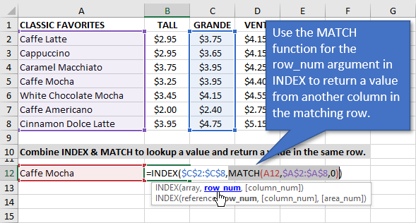
Combining INDEX and MATCH
By combining the INDEX and MATCH functions, we have a comparable replacement for VLOOKUP.
To write the formula combining the two, we use the MATCH function to for the row_num argument.
In the example above I used a 4 for the row_num argument for INDEX. We can just replace that with the MATCH formula we wrote.
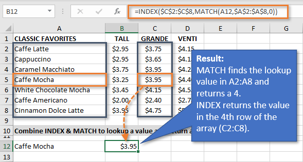
The MATCH function returns a 4 to the row_num argument in INDEX. INDEX then returns the value of that cell, the 4th row in the array (range).
The result is $3.95, the price of the Caffe Mocha size Grande.
Here is a simple guide to help you write the formula until you've practiced enough to memorize it.
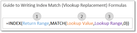
Again, you can think of MATCH as the VLOOKUP. It just returns a row number to INDEX. INDEX then returns the value of the cell in a separate column.
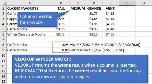
VLOOKUP versus INDEX MATCH
Could we have accomplished the same thing with VLOOKUP in our example? Yes. But again, the advantage of using the INDEX MATCH formulas is that it's less susceptible to breaking when the spreadsheet changes.
Inserting and Deleting Columns
If, for example, we were to add a new cup size to our coffee menu and insert a column between Tall and Grande, our Vlookup formula would return the wrong result. This happens because Grande is now the 4th column, but the index number for VLOOKUP is still 3.
You can also use the MATCH function with VLOOKUP to prevent these types of errors. However, VLOOKUP still can't perform a lookup to the left.
Look to the Left
In this case, the items could be to the right of the prices and INDEX MATCH would still work.
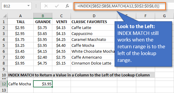
In fact, we don't even have to rewrite the formula if we move the columns around.
Matching Both Row and Column Numbers
I just want to quickly note that you can use two MATCH functions inside INDEX for both the row and column numbers.
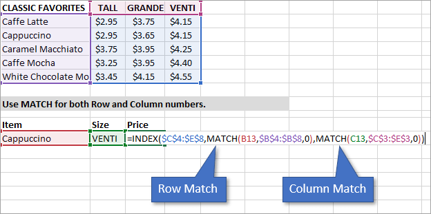
In this example, the return range spans multiple rows and columns C4:E8.
We can use MATCH for lookups both vertically or horizontally. So, the MATCH function can be used twice inside INDEX to perform a two-way lookup. Looking up both the item name and price column.
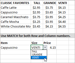
I've added drop-downs (data validation lists) for both the Item and Size to make this an interactive price calculator. When the user selects the item and size, the INDEX MATCH MATCH formula will automatically perform the lookups and return the correct price.
The Most Common Error with INDEX MATCH Formulas
The most common error you will probably see when combining INDEX and MATCH functions is the #REF error.
This is usually caused when the return range in INDEX is a different size from the lookup range in MATCH. In the image below, you can see that the MATCH range includes row 8, while the INDEX range only goes up to row 7. When the specified criteria can't be found because of the misalignment, this will cause the formula to return an error that says #REF.
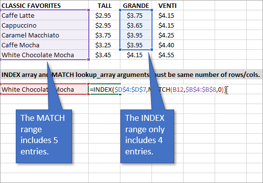
To fix the error, you can simply expand the smaller range to match the larger. In this case, we would change the INDEX range to end at cell D8 instead of D7.
INDEX MATCH will also return the #N/A error when a value is not found, just like VLOOKUP.
Using Excel Tables to Reduce Errors
The example above was easy enough to spot and fix because the data set is so small. When working with larger data sets the mismatch can occur more often because there are blank cells in the data. One workaround for that is to reference Tables instead of ranges. Here is a tutorial that explains more about Excel Tables and Structured Reference Formulas.
Conclusion
INDEX MATCH can be difficult to understand at first. I encourage you to practice with the example file and you'll have this formula committed to memory in no time.
The new XLOOKUP function is an alternative to VLOOKUP and INDEX MATCH that is easier to write. It will just be limited by availability and backward compatibility in the near future.
Please leave a comment below with questions or suggestions.
📤How to Download ebooks: https://www.evba.info/2020/02/instructions-for-downloading-documents.html?m=1


Leave a Comment