Power Query Challenge – Joining two tables fully

Power Query Challenge – Joining two tables fully

by MF

Left Outer + Right Anti = A better Full Join

A sample file is available below.

If you prefer reading to watching, please continue to read this post.

The situation:

I have two tables.  One is Sales Table; One is Traffic Table.  What we need to do is to combine them into a single fact table.

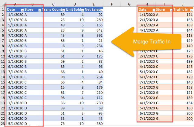
With Power Query, it is an easy job.  We can merge the two tables with Left Outer Join!

BUT… If we do that with Left Outer Join, we will miss some data points.  The following screenshot depicts the situation:

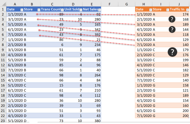
Those traffic records with “?” do not have a matching record in the Sales table.  As a result, those traffic records are missed in the output, and most of the time without any notice/warning…  

In ideal world, every store should have sales every day.  However in real world, there may be zero-sales days… sad but true.  In those days, we had visitors (Traffic In) but no sales, which is no good.  In this case, if we use Left Outer Join, we will miss out those data with Traffic but no sales.  

You may suggest we use the Traffic table as the anchor table to merge sales data to it, it will solve the problem (by using Right Outer Join; or swap the order of the tables).  Well, that’s only true when all stores have traffic data.  Nevertheless, only a few stores (in our example, 3 out of 8) have traffic data.

Thus we need a Full Join to return a result like this:

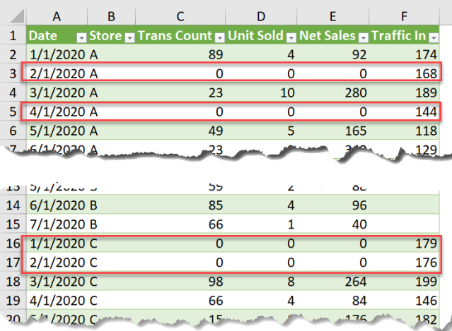
This, however, cannot be achieved directly with Full Outer Join in Power Query.  We need to achieve this with extra steps.  Let’s see how we do it with Power Query!

You may download a sample file to follow along.
Sample File - Start
Sample File - Finish

Load the two tables into Power Query

Select any cell in the Sales table

1. Go to Data tab
2. Select From Table/Range

In the Power Query Editor

1. Under Home Tab –> Close & Load
2. Close & Load to…
3. Only Create Connection
4. OK

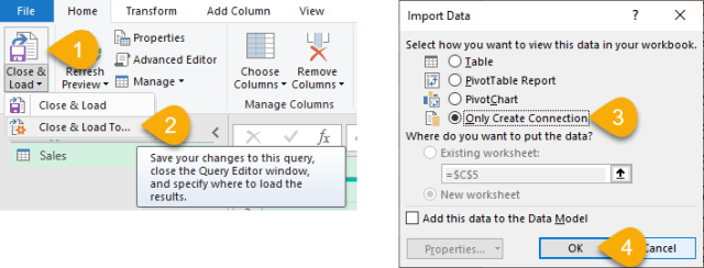
Repeat the steps above for Traffic table.

Edit the Queries

Now we should have the two queries loaded to connection only, as you can see in the Queries and Connections pane.  Right click the Sales query and Edit…

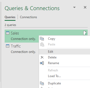
First (failed) attempt – Merge Queries with Full Outer Join

If you have experience with merging queries in Power Query, Full Outer Join should be your top-of-mind solution for this problem.  Nevertheless, it’s not a convenient way as the layout of the output will not be what you want…

Let’s have a look!

Select the Sales query

1. Go to the Home tab of the Power Query Editor
2. Merge Queries
3. Merge Queries (Note: This step is not necessary if we are working on the same query)
4. On the first (Sales) table, select the matching columns 
5. Select Traffic as the second table
6. Select the matching columns (in the right order)
7. Select Full Outer Join (all rows from both)
8. OK

Now we should have a new column called Traffic…

Click the double arrows icon in the column header, and then

1. Check Traffic In only
2. Un-check the box
3. OK

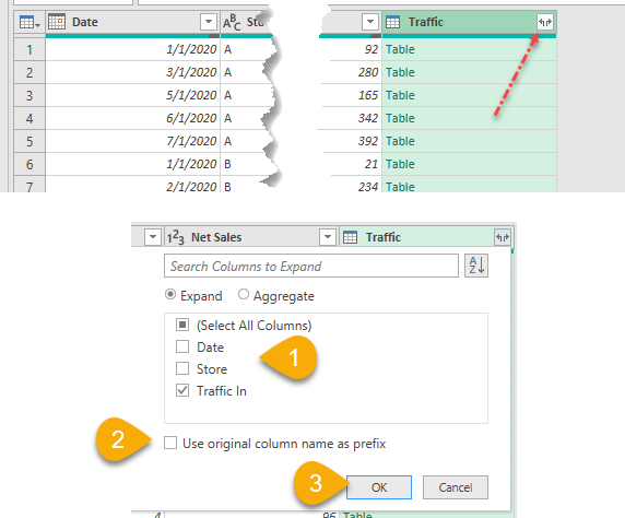
Here we go!

We have the Traffic correctly mapped to the Sales table.  From row 53 to 56, the four records with traffic but no sales are displayed there.  However nothing is under the Date and Store columns…

Wait… what if we go back one step and check also the “Date” and “Store“?

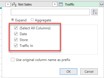
Well, although we get the Date and Store information as expected, we’d also got two extra columns across the entire merged table…

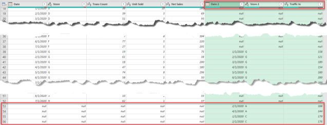
This is obviously not an ideal layout.  Who wants two columns for the same attributes?

We will need many tedious steps to convert this layout back to normal.  Therefore I am going to do it with another approach, which is exactly the topic of today. 

Second attempt – Left Out Join + Right Anti Join followed by Append

A. Merge Queries with Left Outer Join

Repeat the Merge Step described above.  But this time we do a Left Outer Join:

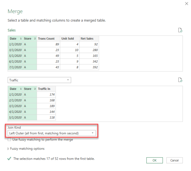
Note: Expand the “Traffic In” column only

B. Duplicate the Sales Query

1. Right click the Sales query on the Queries pane
2. Select Duplicate

On the Query Settings on the right,

1. Rename it to “TrafficWithNoSales“
2. Delete the steps “Expanded Traffic” and “Merged Queries” by clicking the x

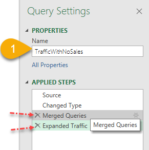
C. Doing a Right Anti Join

1. Select the TrafficWithNoSales query
2. Go to Home tab
3. Merge Queries

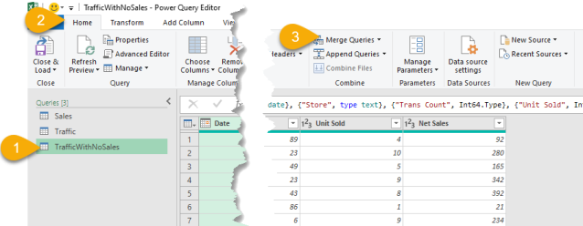
On the Merge queries dialog box:

1. Select the matching columns
2. Select Traffic
3. Select the matching columns (in order)
4. Select Right Anti (rows only in second)
5. OK

The result we have should contain only one row!  All the TrafficWithNoSales records are stored in the “Table” under the Traffic column.

Click the “Table” to open it.

Yeah… We’ve got a table showing the records where we have Traffic but no sales.

D. Append the “Sales” and “TrafficWithNoSales” queries

1. Select the Sales query
2. Go to Home tab
3. Append Queries
4. Select “TrafficWithNoSales“
5. OK

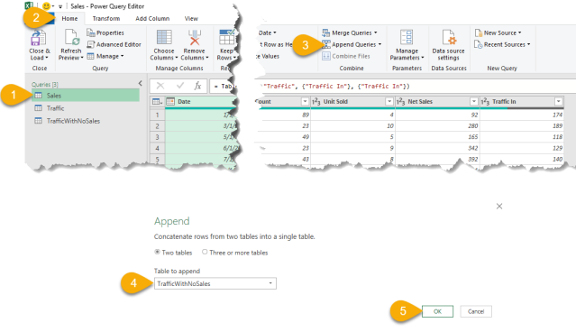
Note: The columns “Date” and “Store” in the two tables must be exactly the same.  Otherwise the Appended result may put them into different columns.  You may need to rename the column headers if required.

Almost there…

Now we have the TrafficWithNoSales records nicely appended to the Sales table merged with traffic data.

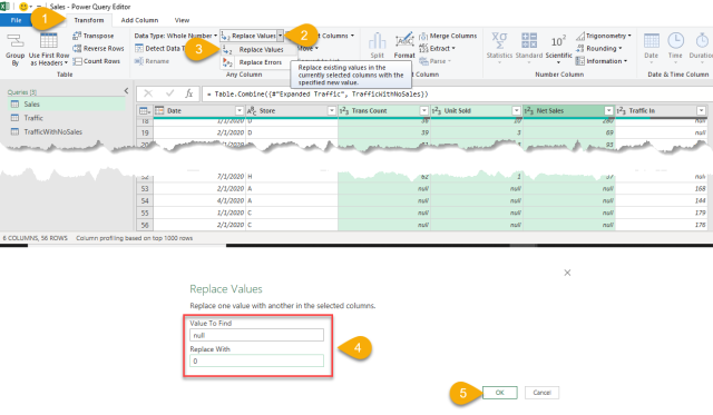
E. Replace null with 0

1. Go to the Transform tab
2. Replace Values
3. Replace Values (Note: this step is not necessary)
4. Replace null with 0
5. OK

F. Final touch – Sort the columns

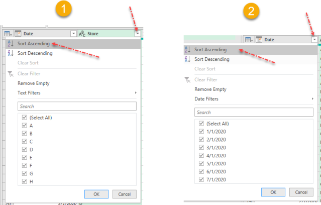
Tip: We may also rename the query to something more meaningful, e.g. Sales with Traffic data

Here we go!  A fully joined table as a result:

Load it to your workbook as you wish.

How do you solve this problem?

Would you do it differently? Please leave your comments below.

#evba #etipfree #eama #kingexcel
📤How to Download ebooks: https://www.evba.info/2020/02/instructions-for-downloading-documents.html?m=1