Creating Currency Converter in Excel [How To]

In the world we live in where almost every country has its own distinct currency and value, we almost always feel a need to convert one currency to another. These days it is easy as we can look for them over the internet and calculate how much a dollar is in terms of Pakistan Rupee. Instead of looking anywhere else we can make it in Excel and it doesn’t take much effort either. So lets toss the coins!

Understanding the concept

For a currency converter to work we don’t need the conversion rates of every currency for every other currency in the world. As the world economics is relative therefore every currency is linked to another and we can find out the conversion rate of two currencies even if we don’t know it directly.

For example if I know the conversion rate of 1 USD to PKR and 1 USD to AED then I can easily find out the conversion rate between 1PKR to AED. Let me explain how it works:

1 USD = 99.8 PKR [Equation 1]

And 1 PKR = 0.01002 USD (1/99.8 = 0.01002)

1 USD = 3.674 AED [Equation 2]

And 1 AED = 0.27218 USD (1/3.674 = 0.27218)

As left hand side of equation 1 and 2 is same therefore we can safely say that right hand sides are also equal to each other. Therefore:

99.8 PKR = 3.674 AED

Now if I want to know how much 1 AED is in terms of PKR I simply have to move 3.674 to the left hand side of the equation:

99.8 PKR x 1/3.674 = 1 AED

As we know 1/3.674 = 0.27218 so putting this value in the equation we get:

99.8 PKR x 0.27218 = 1AED

Therefore:

1 AED = 27.163 PKR

So we understood that even if we have exchange rates of just one currency for all the others we can still find the exchange rate between any two currencies of the world. And this is exactly the concept I will be using in our currency converter in Excel. So lets open the cash box!

Currency Converter Step-by-step

We need updated currency exchange rates that we can use. There are number of ways to get it done but the one that worked for me best is by using Excel’s built-in features. If this fails then the rest of the process is futile. So to have a reliable workbook I will be going with Excel’s existing connections.

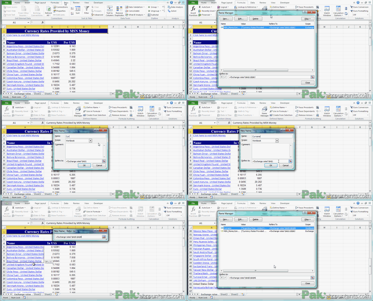
Step 1: Open Excel and go to Data tab and click Existing connections button.

Step 2: From the popup select MSN MoneyCentral Investor currency rates and click open button

Step 3: Excel will ask if you want to pull the information in the same worksheet or a new one. Let it be existing worksheet with the cell address being the default too.

Step 4: Before you click OK button click properties.

Step 5: Activate the option Refresh every _____ minutes and type in the number of minutes after which Excel will refresh the sheet automatically to get the latest rates. Lets make it 5 minutes.

Step 6: Tick the option just under it that says Refresh data when opening file. This way file will have latest data every time you open it at the start of the day. Click OK button to close the box. It will take some time to fetch the data depending upon internet speed.

Step 7: Once the data is imported rename the worksheet to Exchange rates.

Following animation walks you through all the 7 steps explained:

Step 8: Select cell A5 to A46 and type Curname in the name box to give name to this range. It will make writing formulas much easier later.

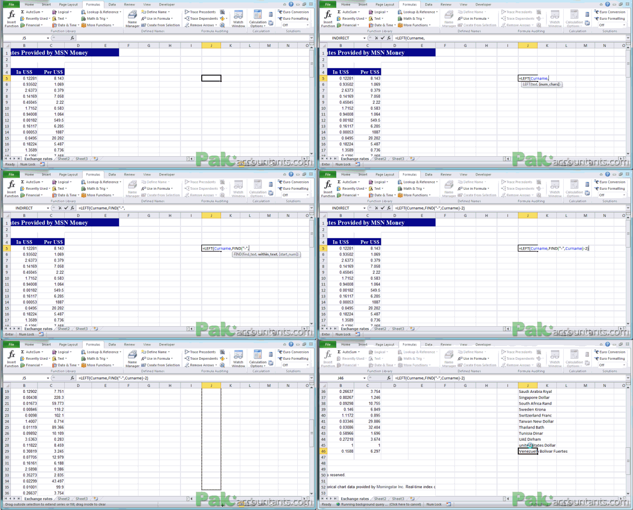
Step 9: Go to cell J5 in the same worksheet and put the following formula and drag the fill handle down to cell J46:

=LEFT(Curname,FIND(“-“,Curname)-2)

This will fetch the currency names leaving the unnecessary string of ” – United states dollar”.

Step 10: Select J5 to J46 and type Curlist in the name box to give name to this range.

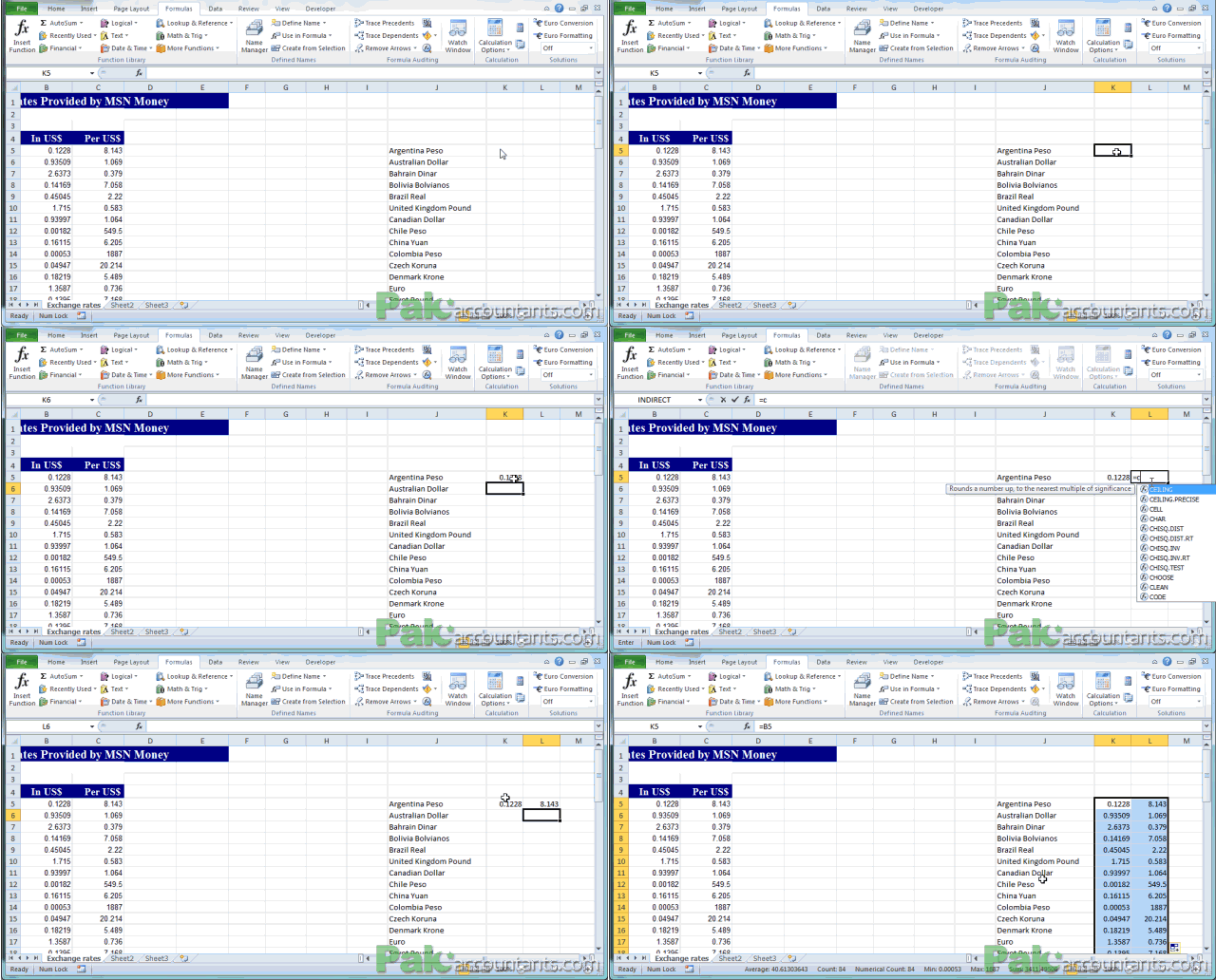
Step 11: Go to cell K5 and type =B5. Hit enter and double click the fill handle. It will fetch the values from column B.

Step 12: Go to cell L5 and type =C5. Hit enter and double click the fill handle. It will fetch another set of values.

Step 13: Select all the cells from J5 to L46 and name it Curtable by typing it in the name box and hitting Enter key on the keyboard.

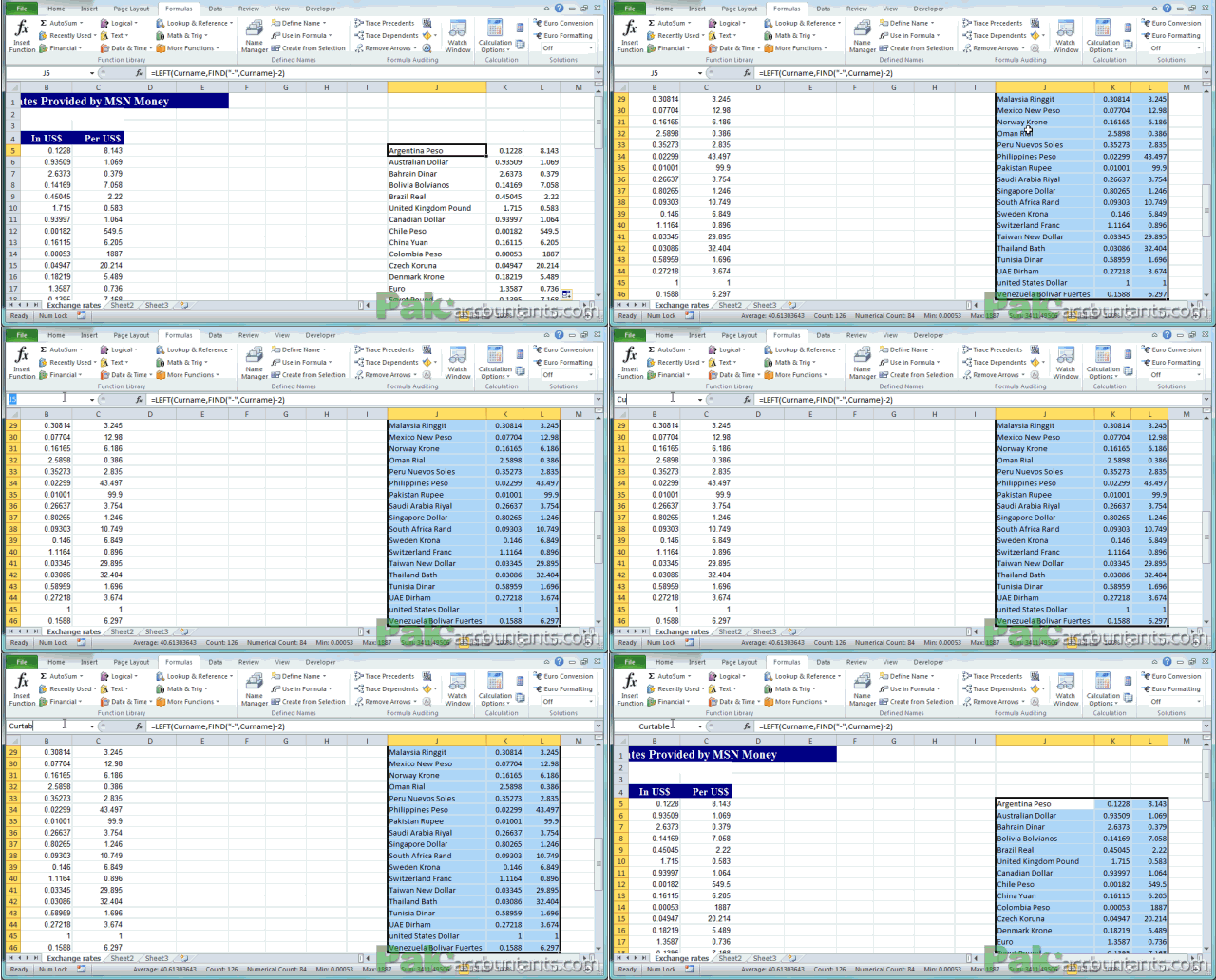
Step 14: Select columns J K and L. Right click on column J and hide all of them to keep the worksheet clean.

Creating currency converter

Now that we have all the basics done, we can proceed with the converter itself to start number crunching

Step 1: Open another worksheet and name it Currency Converter. Type Convert in cell A2 and To in cell A3.

Step 2: Go to cell B2 and click Data tab > Data validation button in data tools group.

Step 3: Under Allow select list and in source type in =Curlist and click OK. This will put all the names of currencies in the form of drop down menu for easy selection.

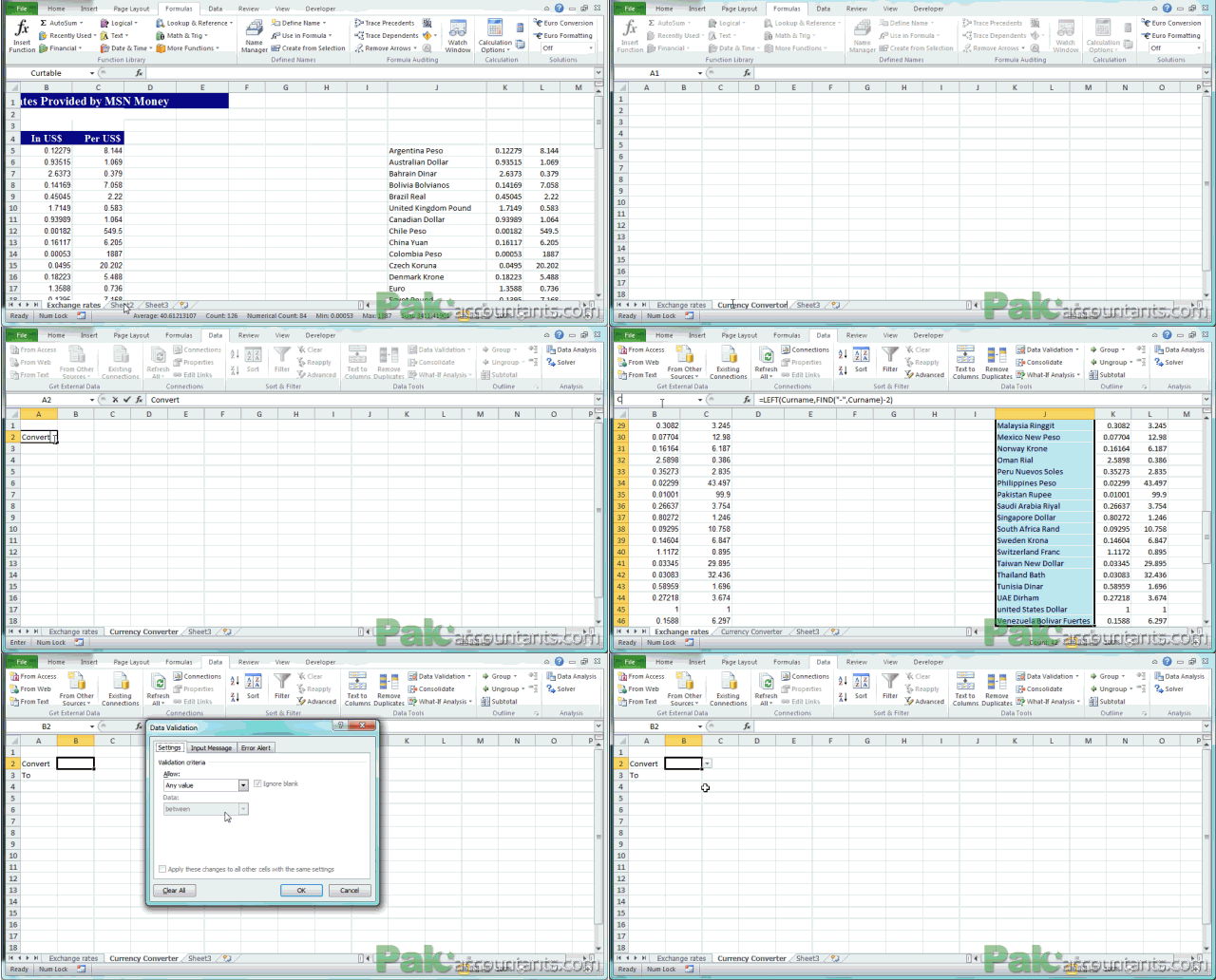
Step 4: Go to cell B3 and repeat Step 3 to get the list.

Step 5: Go to Currency Converter worksheet and in cell C3 put this formula:

=VLOOKUP(B3,curtable,3,FALSE)*VLOOKUP(B2,curtable,2,FALSE)

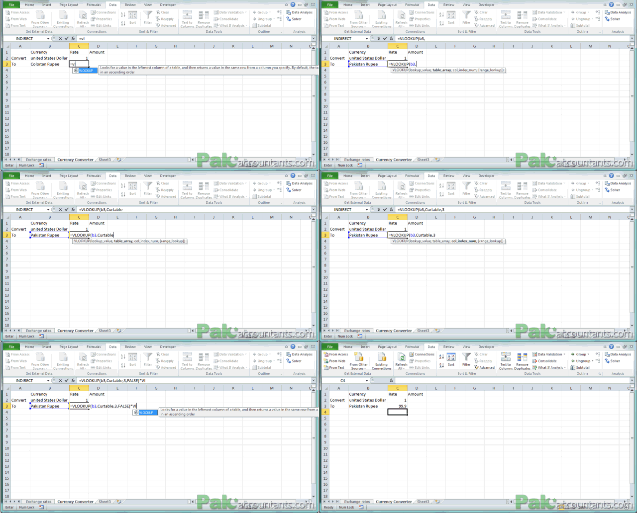
This is the formula based on the concept we discussed in the beginning. Now let make final few touches and its all done.

Step 6: Go to cell D3 and put this formula:

=D2*C3

This will help you calculate the total amount for any given amount in another currency you want to convert.

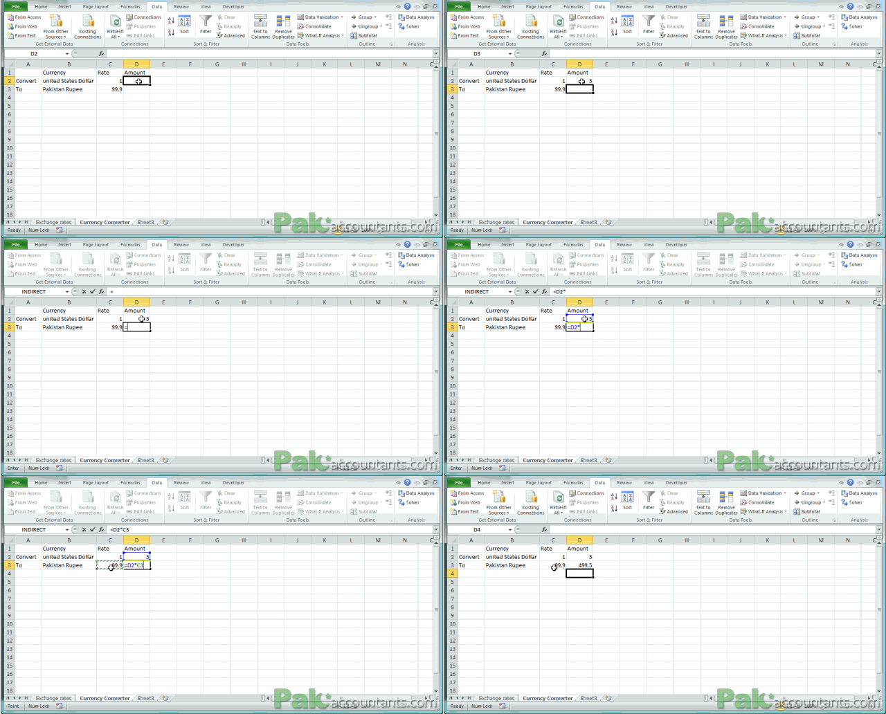
And DONE!

So lets summarize what we learnt:

1. We learnt how finance and currency works even if we have one base currency to calculate other rates.
2. We successfully imported conversion rates using built-in feature that was hidden under the less known group.
3. We learn how to separate part of text out of the whole string in the cell using LEFT and FIND functions.
4. We used named ranges, learnt how to make them and to use them in formula to make the whole process easier.
5. And lastly we used VLOOKUP function to get the converter running and munching numbers!

#evba #etipfree #eama #kingexcel
📤How to Download ebooks: https://www.evba.info/2020/02/instructions-for-downloading-documents.html?m=1