Search and Highlight Data Using Conditional Formatting

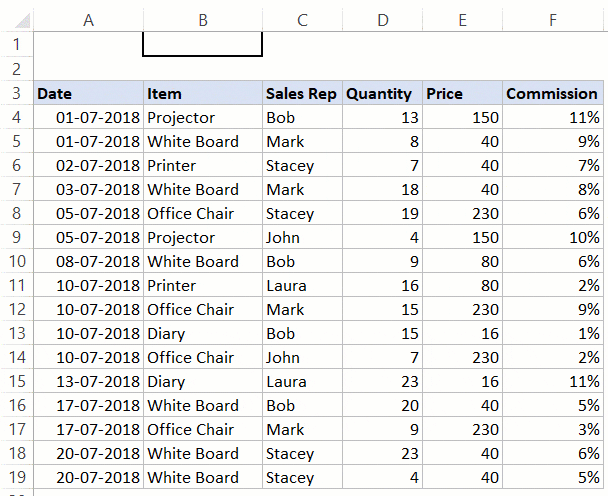
For example, suppose you have a dataset as shown below (in the image). It has columns for Product Name, Sales Rep, and Country.

Now you can use conditional formatting to search for a keyword (by entering it in cell C2) and highlight all the cells that have that keyword.

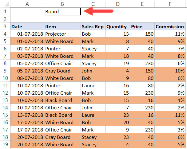
Something as shown below (where I enter the item name in cell B2 and press Enter, the entire row gets highlighted):

In this tutorial, I will show you how to create this search and highlight functionality in Excel.

Later in the tutorial, we will go a bit advanced and see how to make it dynamic (so that it highlights while you’re typing in the search box).

Click here to download the example file and follow along.

This Tutorial Covers:

• Search and Highlight Matching Cells
• Search and Highlight Rows with Matching Data
• Search and Highlight Rows (based on Partial Match)
• Dynamic Search and Highlight Functionality (Highlights as you type)

Search and Highlight Matching Cells

In this section. I will show you how to search and highlight only the matching cells in a dataset.

Something as shown below:

Here are the steps to search and highlight all the cells that have the matching text:

1. Select the dataset on which you want to apply Conditional Formatting (A4:F19 in this example).
2. Click the Home tab.
3. In the Styles group, click on Conditional Formatting.
4. In the drop-down options, click on New Rule.
   
5. In the ‘New Formatting Rule’ dialog box, click on the option ‘Use a formula to determine which cells to format’.
6. Enter the following formula: =A4=$B$1
7. Click on ‘Format..’ button.
8. Specify the formatting (to highlight cells that match the searched keyword).
9. Click OK.

Now type anything in cell B1 and press enter. It will highlight the matching cells in the dataset that contain the keyword in B1.

How does this work?

Conditional Formatting gets applied whenever the formula specified in it returns TRUE.

In the above example, we check each cell using the formula =A4=$B$1

Conditional Formatting checks each cell and verifies it the content in the cell is the same as that in cell B1. If it’s the same, the formula returns TRUE and the cell gets highlighted. If it isn’t the same, the formula returns FALSE and nothing happens.

Click here to download the example file and follow along.

Search and Highlight Rows with Matching Data

If you want to highlight the entire row instead of just the matching cells, you can do that by tweaking the formula a little.

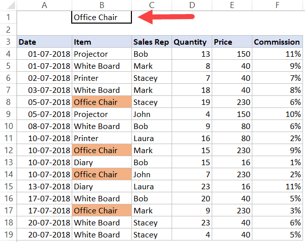
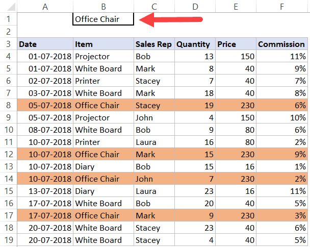
Below is an example where the entire row gets highlighted if the product type matches the one in cell B1.

Here are the steps to search and highlight the entire row:

1. Select the dataset on which you want to apply Conditional Formatting (A4:F19 in this example).
2. Click the Home tab.
3. In the Styles group, click on Conditional Formatting.
4. In the drop-down options, click on New Rule.
   
5. In the ‘New Formatting Rule’ dialog box, click on the option ‘Use a formula to determine which cells to format’.
6. Enter the following formula: =$B4=$B$1
7. Click on ‘Format..’ button.
8. Specify the formatting (to highlight cells that match the searched keyword).
9. Click OK.

The above steps would search for the specified item in the dataset, and if it finds the matching item, it will highlight the entire row.

Note that this will only check for the item column. If you enter a Sales Rep name here, it will not work. If you want it to work for Sales Rep name, you need to change the formula to =$C4=$B$1

Note: The reason it highlights the entire row and not just the matching cell is that we have used a $ sign before the column reference ($B4). Now when conditional formatting analyzes cells in a row, it checks whether the value in column B of that row is equal to the value in cell B1. So even when it’s analyzing A4 or B4 or C4 and so on, it’s checking for B4 value only (as we have locked column B by using the dollar sign).

You can read more about absolute, relative and mixed references here.

Search and Highlight Rows (based on Partial Match)

In some cases, you may want to highlight rows based on a partial match.

For example, if you have items such as White Board, Green Board, and Gray Board, and you want to highlight all these based on the word Board, then you can do this using the SEARCH function.

Something as shown below:

Here are the steps to do this:

1. Select the dataset on which you want to apply Conditional Formatting (A4:F19 in this example).
2. Click the Home tab.
3. In the Styles group, click on Conditional Formatting.
4. In the drop-down options, click on New Rule.
   
5. In the ‘New Formatting Rule’ dialog box, click on the option ‘Use a formula to determine which cells to format’.
6. Enter the following formula: =AND($B$1<>””,ISNUMBER(SEARCH($B$1,$B4)))
7. Click on ‘Format..’ button.
8. Specify the formatting (to highlight cells that match the searched keyword).
9. Click OK.

How does this work?

• SEARCH function looks for the search string/keyword in all the cells in a row. It returns an error if the search keyword is not found, and returns a number if it finds a match.
• ISNUMBER function converts the error into FALSE and the numeric values into TRUE.
• AND function checks for an additional condition – that cell C2 should not be empty.

So now, whenever you type a keyword in cell B1 and press Enter, it highlights all the rows that have the cells that contain that keyword.

Bonus Tip: If you want to make the search case sensitive, use the FIND Function instead of SEARCH.

Click here to download the example file and follow along.

Dynamic Search and Highlight Functionality (Highlights as you type)

Using the same Conditional Formatting tricks covered above, you can also take it a step further and make it dynamic.

For example, you can create a search bar where the matching data gets highlighted as you’re typing in the search bar.

Something as shown below:

This can be done using ActiveX controls and can be a good functionality to use when creating reports or dashboards.

#evba #etipfree #kingexcel
📤You download App EVBA.info installed directly on the latest phone here : https://www.evba.info/p/app-evbainfo-setting-for-your-phone.html?m=1