How to Delete Every Other Row in Excel (or Every Nth Row)

This Tutorial Covers:

• Delete Every Other Row By Filtering the Dataset (Using Formula)
• Delete Every Nth Row By Filtering the Dataset (Using Formula)
• Automatically Delete Every Other Row (or Nth row) using VBA Macro (Quick Method)
• Delete Every Other Column (or Every Nth Column)
  • Delete Alternate Columns Using Formulas and Sort Method
  • Delete Alternate Columns Using VBA

Delete Every Other Row By Filtering the Dataset (Using Formula)

If you could somehow filter all the even rows or the odd rows, it would be super easy to delete these rows/records.

While there is no inbuilt feature to do this, you can use a helper column to first divide the rows in to odd and even, and then filter based on the helper column value.

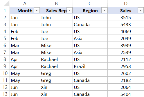
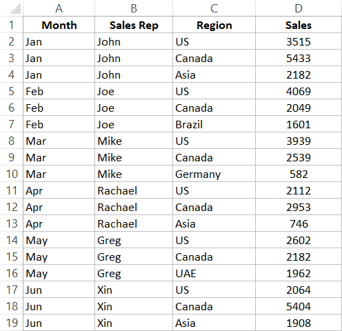
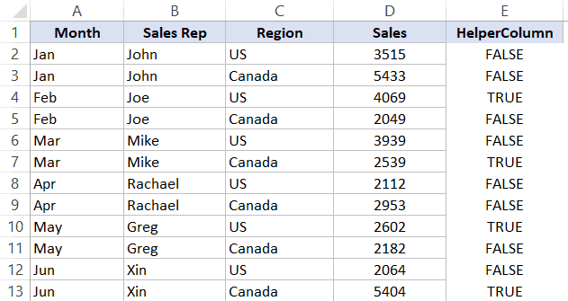
Suppose you have a dataset as shown below, which has sales data for each sales rep for two regions (the US and Canada) and you want to delete the data for Canada.

Below are the steps to first filter and then delete every other row (which has data for Canada):

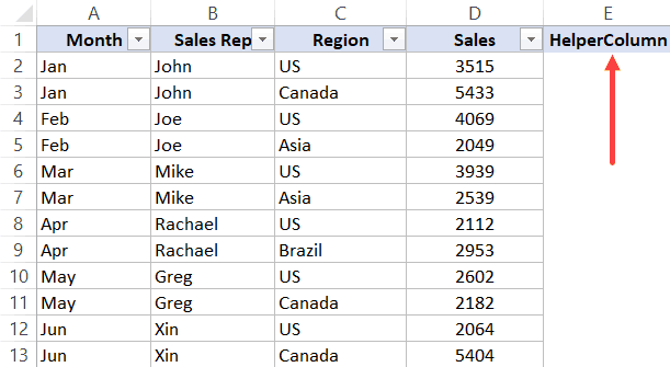
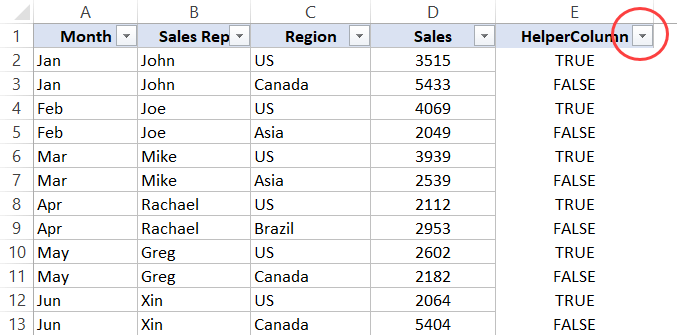
1. In the cell adjacent to the last column header, enter the text HelperColumn (or any header text that you want the helper column to have)
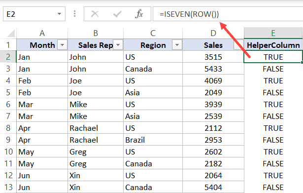
2. In the cell below the helper column header, enter the following formula: =ISEVEN(ROW()). Copy this formula for all the cells. This formula returns TRUE for all even rows and FALSE for all ODD rows
3. Select the entire dataset (including the cells where we entered the formula in the above step).
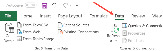
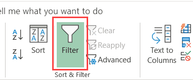
4. Click the Data tab
5. Click the Filter icon. This will apply a filter to all the headers in the dataset
6. Click the Filter icon in the HelperColumn cell.
7. Deselect the TRUE option (so only the FALSE Option is selected)
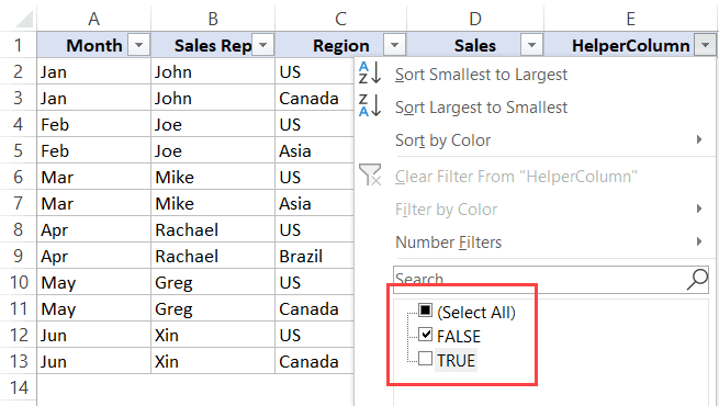
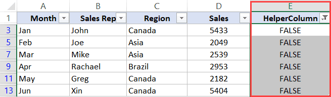
8. Click OK. This will filter the data and only show those records where the HelperColumn value is FALSE.
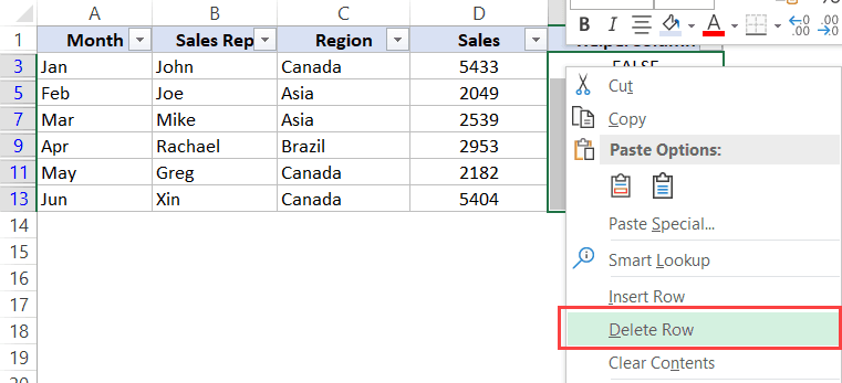
9. Select all the filtered cells in the helper column (excluding the header)
10. Right-click on any of the selected cells and click on ‘Delete Row’
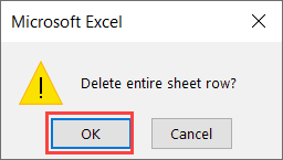
11. In the dialog box that opens, click on OK. This will delete all the visible records and you will only see the header row as of now.
12. Click the Data tab and then click the Filter icon. This will remove the filter and you will be able to see all the remaining records.

The above steps filter every second row in the dataset and then deletes those rows.

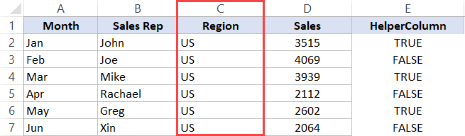
Don’t worry about the helper column values at this stage. The resulting data has only the rows for the US  and all the Canada rows are deleted. You can delete the helper column now.

In case you want to delete every other row starting from the first row onwards, select the TRUE option in step 7 and deselect the FALSE option.

Note: When you delete the rows in Excel using the above method, it also deletes any data that you may have in the entire (apart from the one in the dataset). When you use this method, make sure you don’t have anything to the left and right of the dataset that you’re deleting.

While the above method is great, it has two drawbacks:

1. It needs to you add a new column (the HelperColumn in our example above)
2. It can be time-consuming if you have to delete alternate rows do this often

Delete Every Nth Row By Filtering the Dataset (Using Formula)

In the above method, I showed you how to delete every other row (alternate row) in Excel.

And you can use the same logic to delete every third or fourth row in Excel as well.

Suppose you have a dataset as shown below and you want to delete all every third row.

The steps to delete every third row are almost the same as the one covered in the above section (for deleting alternate rows). The only difference is in the formula used in Step 2.

Below are the steps to do this:

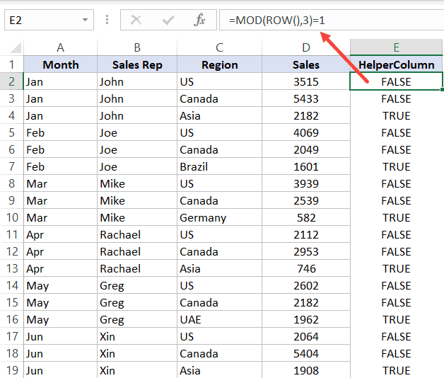
1. In the cell adjacent to the last column header, enter the text HelperColumn (or any header text that you want the helper column to have)
2. In the cell below the helper column header, enter the following formula: =MOD(ROW(),3)=1. This formula returns TRUE for every third row and FALSE for every other row.
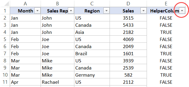
3. Select the entire dataset (including the cells where we entered the formula in the above step).
4. Click the Data tab
5. Click the Filter icon. This will apply a filter to all the headers in the dataset
6. Click the Filter icon in the HelperColumn cell.
7. Deselect the TRUE option (so only the FALSE Option is selected)
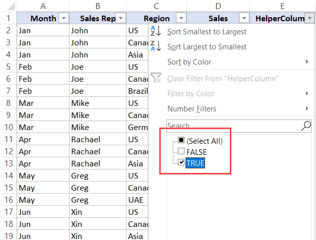
8. Click OK. This will filter the data and only show those records where the HelperColumn value is FALSE.
9. Select all the cells in the helper column
10. Right-click on any of the selected cells and click on Delete Row
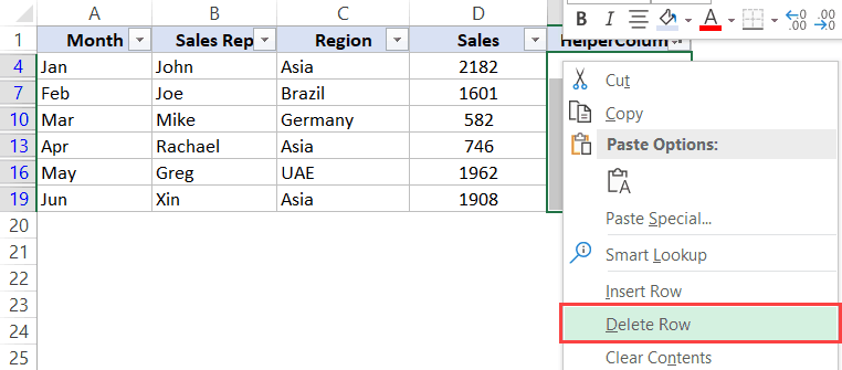
11. In the dialog box that opens, click on OK. This will delete all the visible records and you will only see the header row as of now.
12. Click the Data tab and then click the Filter icon. This will remove the filter and you will be able to see all the remaining records.

The above steps would delete every third row from the dataset and you would get the resulting data as shown below.

Don’t worry about the helper column values at this stage. You can delete the helper column now.

The formula used in Step 2 uses the MOD function – which gives the remainder when one number is divided by the other. Here I have used the ROW function to get the row number and it’s divided by 3 (because we want to delete every third row).

Since our dataset starts from the second row onwards (i.e., row #2 contains the first record), I use the following formula:=MOD(ROW(),3)=1

I am equating it to 1 and for every third row, the MOD formula will give the remainder as 1.

You can adjust the formula accordingly. For example, if your dataset’s first record starts from third-row onwards, the formula would be =MOD(ROW(),3)=2

Automatically Delete Every Other Row (or Nth row) using VBA Macro (Quick Method)

If you have to delete every other row (or every nth row) quite often, you can use a VBA code and have it available in ṭhe Quick Access Toolbar. This will allow you to quickly delete alternate rows with a single click.

Below is the code that first asks you to select the range in which you want to delete alternate rows, and then delete every second row in the selected dataset.

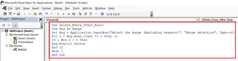
Sub Delete_Every_Other_Row()
Dim Rng As Range
Set Rng = Application.InputBox("Select the Range (Excluding headers)", "Range Selection", Type:=8)
For i = Rng.Rows.Count To 1 Step -2
If i Mod 2 = 0 Then
Rng.Rows(i).Delete
End If
Next i
End Sub

When you run the above code, it will first ask you to select the range of cells. Once you have made the selection, it will go through each row and delete every second row.

If you want to delete every third row instead, you can use the below code:

Sub Delete_Every_Third_Row()
Dim Rng As Range
Set Rng = Application.InputBox("Select the Range (Excluding headers)", "Range Selection", Type:=8)
For i = Rng.Rows.Count To 1 Step -3
If i Mod 3 = 0 Then
Rng.Rows(i).Delete
End If
Next i
End Sub

Where to put this VBA macro code?

You need to place this code in a regular module in the VB editor in Excel.

Below are the steps to open the Vb Editor, add a module and place the code in it:

1. Copy the above VBA code.
2. Go to the Developer tab.
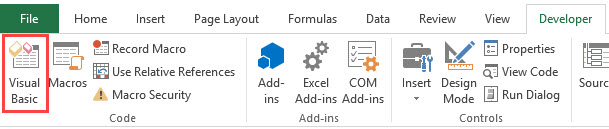
3. Click on Visual Basic.
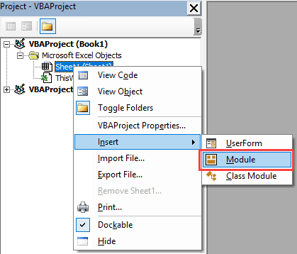
4. In the VB Editor, right-click on any of the workbook objects.
5. Go to Insert and click on Module.
6. In the module, paste the above VBA code.
7. Close the VB Editor.

Once you have the code in the VB Editor, you can use the following methods to run the code:

• Run a Macro from the VB Editor (by clicking on the green play button in VB Editor toolbar)
• By placing the cursor on any line in the code and using the F5 key
• By assigning the macro to a button/shape
• By adding the macro to the Quick Access toolbar

If you have to do this often, you can consider adding the VBA code to the Personal Macro Workbook. This way, it will always be available to you for use in all the workbooks.

When you have a VBA code in a workbook, you need to save it as a macro-enabled filed (with the .XLSM extension)

Note: Since any changes made by the VBA code are irreversible, it’s best to first make a back-up copy of the workbook/worksheet and then run this code.

Delete Every Other Column (or Every Nth Column)

Deleting every alternate row or every third/fourth row is made easy as you can use the filter option. All you have to do is use a formula that identifies alternate rows (or every third/fourth row) and filters these rows.

Unfortunately, this same methodology won’t work with columns – as you can not filter columns the way you filter rows.

So, if you have to delete every other column (or every third/fourth/Nth column), you need to be a little more creative.

In this section, I will show you two methods you can use to delete every other column in Excel (and you can use the same method to delete every third/fourth/Nth column if you want).

Delete Alternate Columns Using Formulas and Sort Method

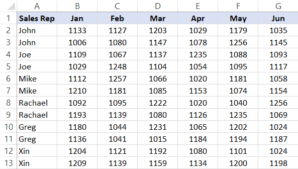
Suppose you have a dataset as shown below and you want to delete every other column (excluding the header column A)

The trick here would be to identify alternate columns using a formula and then sort the columns based on that formula. Once you have the sorted columns together, you can manually select and delete this.

Below are the steps to delete every other column in Excel:

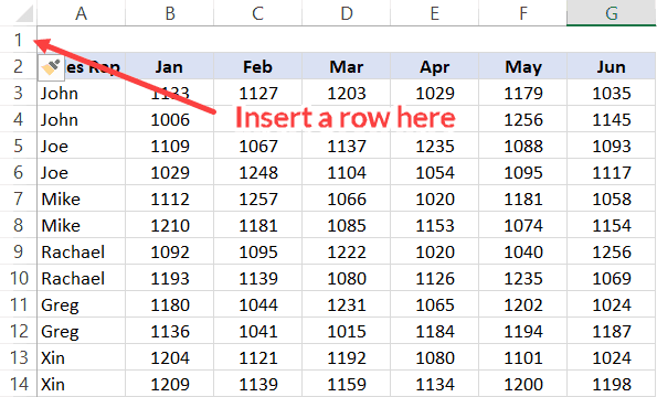
1. Insert a row above the header row (right-click on any cell in the header, click on Insert and then click on Entire row option)
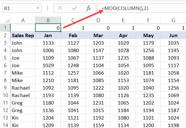
2. Enter the following formula in the cell above the left-most column in the dataset and copy for all cells: =MOD(COLUMN(),2)
3. Convert the formula values to numbers. To do this, copy the cells, right-click and go to Paste Special –> Paste values.
4. Select the entire dataset (excluding any headers in the column). In this example, I have selected B1:G14 (and NOT column A)
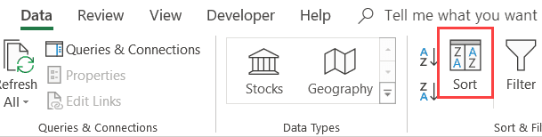
5. Click the Data tab
6. Click on the Sort icon
7. In the Sort dialog box, make the following changes:
   • Click on ‘Options’ button and in the dialog box that opens, click on ‘Sort left to right’ and then Click Ok
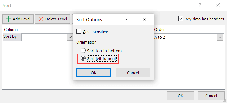
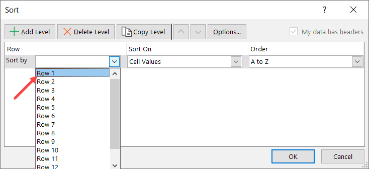
   • In the Sort by drop-down, select Row 1. This is the row that has the formula results
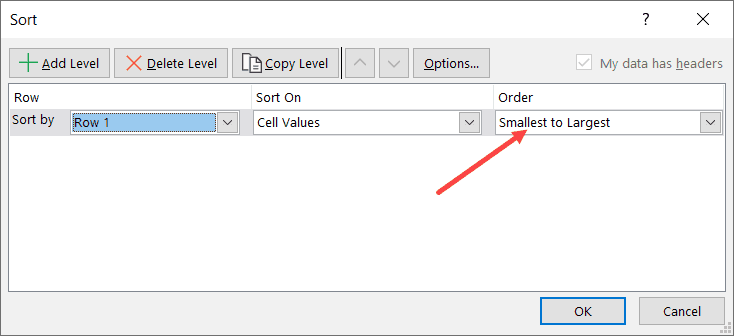
   • In the Order drop-down, select Smallest to Largest.
8. Click OK

The above steps sort all the columns and bring all the alternate columns together at one place (at the end).

Now you can select all these columns (for which the formula value is 1), and delete these.

Although this is not the best solution, it still gets the work done.

In case you want to delete every third column or every fourth column, you need to adjust the formula accordingly.

Delete Alternate Columns Using VBA

Another quick way to delete alternate columns is to use the below VBA code:

Sub Delete_Every_Other_Column()
Dim Rng As Range
Set Rng = Application.InputBox("Select the Range (Excluding headers)", "Range Selection", Type:=8)
For i = Rng.Columns.Count To 1 Step -2
If i Mod 2 = 0 Then
Rng.Columns(i).Delete
End If
Next i
End Sub

The above code asks you to select a range of cells which has the columns. Here you need to select the columns excluding the one which has the header.

Once you have specified the range of cells with the data, it will use a For Loop and delete every other column.

In case you want to delete every third column, you can use the code below (and adjust accordingly to delete the Nth column)

Sub Delete_Every_Third_Column()
Dim Rng As Range
Set Rng = Application.InputBox("Select the Range (Excluding headers)", "Range Selection", Type:=8)
For i = Rng.Columns.Count To 1 Step -3
If i Mod 3 = 0 Then
Rng.Columns(i).Delete
End If
Next i
End Sub

The steps on where to place this VBA code and how to use it covered in the above section titled – “Automatically Delete Every Other Row (or Nth row) using VBA Macro (Quick Method)”

Hope you found this Excel tutorial useful.

#evba #etipfree #kingexcel
📤You download App EVBA.info installed directly on the latest phone here : https://www.evba.info/p/app-evbainfo-setting-for-your-phone.html?m=1