Find the Last Occurrence of a Lookup Value a List in Excel

Recently, I was working on setting the agenda for a meeting.

I had a list in Excel where I had a list of people and the dates on which they acted as the ‘Meeting Chair’.

Since there was repetition in the list (which means that a person has been Meeting Chair multiple times), I also needed to know when was the last time a person acted as the ‘Meeting Chair’.

This was because I had to ensure someone who recently chaired was not assigned again.

So I decided to use some Excel Function magic to get this done.

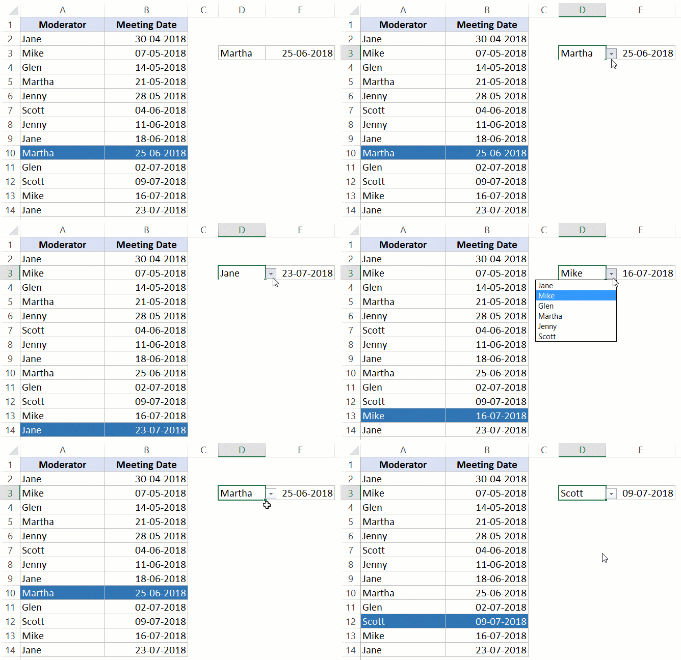
Below is the final result where I am able to select a name from the drop-down and it gives me the date of the last occurrence of that name in the list.

If you have a good understanding of Excel Functions, you would know that there is no one Excel function that can do this.

But you are in the Formula Hack section, and here we make the magic happens.

In this tutorial, I’ll show you three ways to do this.

This Tutorial Covers:

• Find the Last Occurrence - Using MAX function
• Find the Last Occurrence - Using LOOKUP function
• Find the Last Occurrence - Using Custom Function (VBA)

Find the Last Occurrence – Using MAX function

Credit to this technique goes to an article by Excel MVP Charley Kyd.

Here is the Excel formula that will return the last value from the list:

=INDEX($B$2:$B$14,SUMPRODUCT(MAX(ROW($A$2:$A$14)*($D$3=$A$2:$A$14))-1))

Here is how this formula works:

• The MAX function is used to find the row number of the last matching name. For example, if the name is Glen, it would return 11, as it’s in the 11 row. Since our list starts from second row onwards, 1 has been subtracted. So the position of the last occurrence of Glen is 10 on our list.
• SUMPRODUCT is used to ensure that you don’t have to use Control + Shift + Enter, as SUMPRODUCT can handle array formulas.
• INDEX function is now used to find the date for the last matching name.

Find the Last Occurrence – Using LOOKUP function

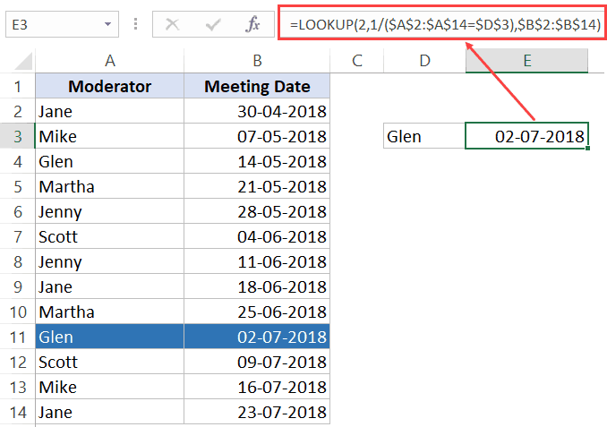
Here is another formula to do the same job:

=LOOKUP(2,1/($A$2:$A$14=$D$3),$B$2:$B$14)

Here is how this formula works:

• The lookup value is 2 (you’ll see why.. keep reading)
• The lookup range is 1/($A$2:$A$14=$D$3) – This returns 1 when it finds the matching name and an error when it doesn’t. So you end up getting an array. For example, of the lookup value is Glen, the array would be {#DIV/0!;#DIV/0!;1;#DIV/0!;#DIV/0!;#DIV/0!;#DIV/0!;#DIV/0!;#DIV/0!;1;#DIV/0!;#DIV/0!;#DIV/0!}.
• The third argument ([result_vector]) is the range from which it gives the result, which are dates in this case.

The reason this formula works is that the LOOKUP function uses the approximate match technique. This means that if it can find the exact matching value, it would return that, but if it can not, it will scan the entire array till the end and return the next largest value which is lower than the lookup value.

In this case, the lookup value is 2, and in our array, we will only get 1’s or errors. So it scans the entire array and returns the position of the last 1 – which is the last matching value of the name.

Find the Last Occurrence – Using Custom Function (VBA)

Let me also show you another way of doing this.

We can create a custom function (also called User Defined Function) using VBA.

The benefit of creating a custom function is that it’s easy to use. You don’t have to worry about creating a complex formula every time, as most of the work happens in the VBA backend.

I have created a simple formula (which is a lot like VLOOKUP formula).

To create a custom function, you need to have the VBA code in the VB Editor. I will give you the code and the steps to place it in the VB Editor in a while, but let me first show you how it works:

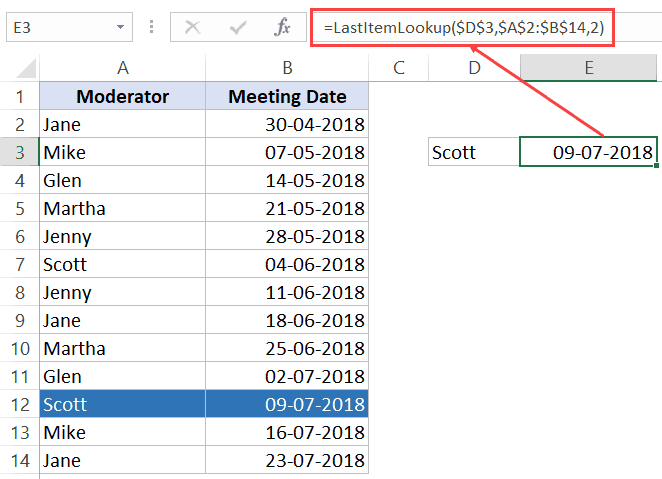
This is the formula that will give you the result:

=LastItemLookup($D$3,$A$2:$B$14,2)

The formula takes three arguments:

• Lookup Value (this would be the name in cell D3)
• Lookup Range (this would be the range that has the names and dates – A2:B14)
• Column Number (this is the column from which we want the result)

Once you have created the formula and put the code in VB Editor, you can use it just like any other regular Excel worksheet functions.

Here is the code for the formula:

'This is a code for a function that finds the last occurrence of a lookup value and returns the corresponding value from the specified column
'Code created by Sumit Bansal (https://trumpexcel.com)
Function LastItemLookup(Lookupvalue As String, LookupRange As Range, ColumnNumber As Integer)
Dim i As Long
For i = LookupRange.Columns(1).Cells.Count To 1 Step -1
If Lookupvalue = LookupRange.Cells(i, 1) Then
LastItemLookup = LookupRange.Cells(i, ColumnNumber)
Exit Function
End If
Next i
End Function

Here are the steps to place this code in the VB Editor:

1. Go to Developer tab.
2. Click on Visual Basic option. This will open the VB editor in the backend.
3. In the Project Explorer pane in the VB Editor, right-click on any object for the workbook in which you want to insert the code. If you don’t see the Project Explorer go to the View tab and click on Project Explorer.
4. Go to Insert and click on Module. This will insert a module object for your workbook.
5. Copy and paste the code in the module window.

Now the formula would be available in all the worksheet of the workbook.

Note that you need to save the workbook in the .XLSM format as it has a macro in it. Also, if you want this formula to be available in all the workbooks you use, you can either save it the Personal Macro Workbook or create an add-in from it.

#evba #etipfree #kingexcel
📤You download App EVBA.info installed directly on the latest phone here : https://www.evba.info/p/app-evbainfo-setting-for-your-phone.html?m=1