Find Largest Value That Meets One or More Criteria

January 03, 2020 Mr King Excel Tips,

Find Largest Value That Meets One or More Criteria

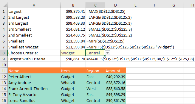
One of the new Office 365 functions added in February 2016 is the MAXIFS function. This function, which is similar to SUMIFS, finds the largest value that meets one or more criteria: You can either hard-code the criterion as in row 7 below or point to cells as in row 9. A similar MINIFS function finds the smallest value that meets one or more criteria.

Amounts appears in D12:D125. To get the Largest, use =MAX($D$12:$D$125). To get the 2nd Largest, use =LARGE($D$12:$D$125,2). To get the 3rd Largest, use =LARGE($D$12:$D$125,3). To get the 3rd Smallest, use =SMALL($D$12:$D$125,3). To get the 2nd Smallest, use =SMALL($D$12:$D$125,2). To get the Smallest, use =MIN($D$12:$D$125). To get the Smallest Widget, use =MINIFS($D$12:$D$125,$B$12:$B$125,"Widget"), To get the Largest with 2 Criteria entered in B8:C8, use =MAXIFS($D$12:$D$125,$B$12:$B$125,B8,$C$12:$C$125,C8)

While most people have probably heard of MAX and MIN, but how do you find the second largest value? Use LARGE (rows 2 and 3) or SMALL (rows 4 and 5).

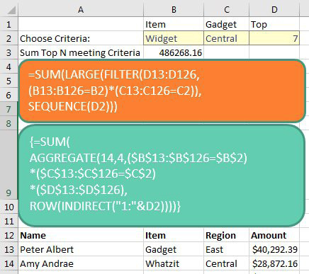
What if you need to sum the top seven values that meet criteria? The orange box below shows how to solve with the new Dynamic Arrays. The green box is the Ctrl+Shift+Enter formula required previously.

Before Dynamic Arrays, you would use: '{=SUM(
AGGREGATE(14,4,($B$13:$B$126=$B$2)
*($C$13:$C$126=$C$2)
*($D$13:$D$126),
ROW(INDIRECT("1:"&D2))))}.
With Dynamic Arrays, the formula is =SUM(LARGE(FILTER(D13:D126,(B13:B126=B2)*(C13:C126=C21)),SEQUENCE(D2)))

#evba #etipfree #kingexcel
📤You download App EVBA.info installed directly on the latest phone here : https://www.evba.info/p/app-evbainfo-setting-for-your-phone.html?m=1