Excel SUMIFS function – Summing up Invoices based on multiple criteria

Excel conditional functions are part of almost every worksheet. The logical test functions help us carry out different operations easily. While discussing SUMIF we learnt to sum the values based on one criteria i.e. date. However, what if we want to sum up the values not only on the basis of date but also the payment status? Now this is a multiple criteria situation and that is where SUMIFS comes into play instead of SUMIF.

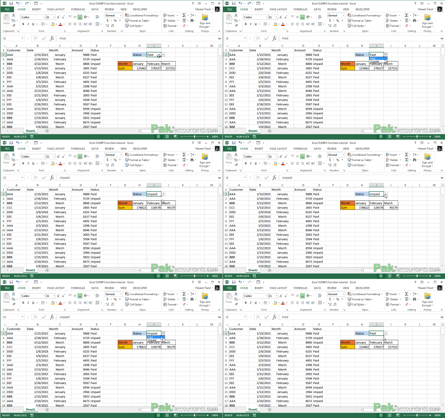
Here is what we will have by the end of this tutorial:

Download Excel Tutorial File

Click here to download the sample excel tutorial file to help you practice the steps in this tutorial

Suppose you have several invoices, some of them unpaid and some paid in different months. We want to sum the invoices based on two criteria i.e. month and status. But lets have a look how SUMIFS function work:

SUMIFS have a following syntax:

SUMIFS(sum_range, criteria_range1, criteria1, [criteria_range2,criteria2], …)

sum_range: the range you like to sum. In our case it is amount column

criteria_range1: first range of criteria. In our case it is month column

criteria1: criteria for the first range. In our case it is January, February or March

criteria_range2: second range of criteria. In our case it is status column

criteria2: criteria for second range. In our case it is either paid or unpaid

 Now lets understand how to get this formula to work.

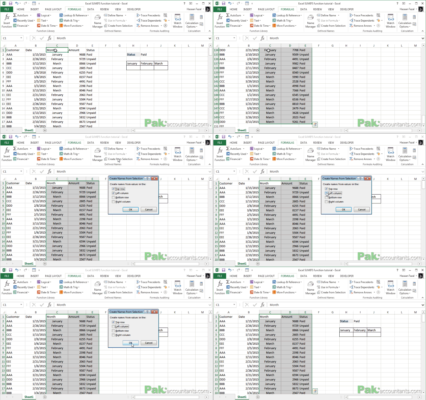
Step 1: Select the Month, Amount and Status columns (with headings and data) and hit Ctrl+Shift+F3 to invoke create names from selection dialogue box. Make sure you have only top row checked. Click OK and now you have names created. It will make writing formula much easier

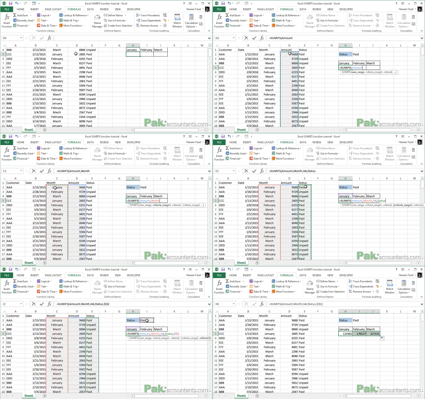
Step 2: Go to cell H5 and put this formula:

=SUMIFS(Amount,Month,H4,Status,$I$2)

I hope its easy to understand the above formula now after the above explanation of function’s syntax and using named ranges. But here are some words:

Amount is the name given to range C2:C150 and is the range we told Excel to sum

Month is the name given to range D2:D150 and is the criteria range for which criteria is mentioned in cell H4 which is a month’s name “January”. It is a relative cell reference and thus if fill handle is moved both row and column is unrestricted and will change.

Status is the name given to range E2:E150 that holds the information if the invoice is paid or not. Criteria for this range is mentioned in cell I2 that can be changed via drop-down.

Step 3: Drag the fill handle to the right from H5 to cell J5 and Excel will calculate the figures for you instantly.

You can sum the values based on status by selecting from drop down menu. If unpaid is selected then you will see the sum of invoices under each month that are still unpaid.

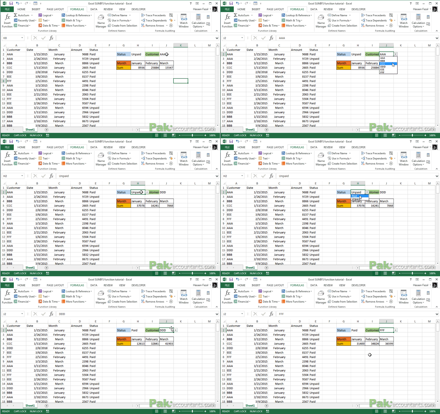
Homework: Add third criteria: Customer

So if we have understood how to apply SUMIFS using multi-criteria capability, we can add another in the formula and sum the invoices based on THREE criteria i.e. month, status and customer. But I am leaving that on you to figure out. Let me know if you need help in the comment box below and we will work it out together.

Just to give you a hint, this is how my attempt looks:

#evba #etipfree #kingexcel
📤You download App EVBA.info installed directly on the latest phone here : https://www.evba.info/p/app-evbainfo-setting-for-your-phone.html?m=1