Customize the Quick Access Toolbar

As I mentioned in Excel 2019: Get Ideas from Artificial Intelligence, the Excel team had not added any new features to the Home tab since January 30, 2007. Ideas is the first feature that was deemed worthy of being on the Home tab.

Even though the Excel team does not think many features are Home-tab-worthy, you can add your favorite features to the Quick Access Toolbar (hereafter called QAT).

I always like asking people what they have added to their QAT. In a Twitter poll in January 2019, I had over 70 suggestions of favorite features that could be added to the QAT.

To me, a "good" addition to the QAT is a command that you use frequently that is not already on the Home tab. Any of the features in the Commands Not In The Ribbon category are candidates if you ever have to use them.

I've suggested the following icons on the QAT:

---

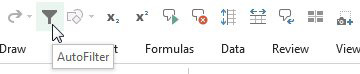
• The AutoFilter icon was used in Excel 2019: Filter by Selection in Excel
• Change Shape in Excel 2019: Old Style Comments Are Available as Notes
• Speak Cells in Excel 2019: Avoid Whiplash with Speak Cells
• Speak Cells on Enter in Excel 2019: A Great April Fool’s Day Trick

Below are more icons that you might want to add to your QAT.

The Easy Way to Add to the QAT

The easiest way to add an icon to the QAT is to right-click the icon in the Ribbon and choose Add to Quick Access Toolbar.

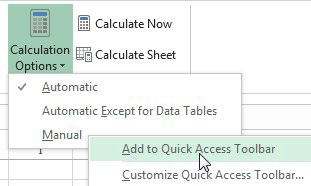
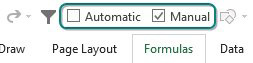
Adding Formulas, Calculation Options, Manual to the QAT gives you a clear indication of when your workbook is in Manual calculation mode:

The Hard Way to Add to the QAT

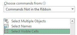
Sometimes, the command you want can not be right-clicked. For example, using Alt+; as a shortcut for Visible Cells in the Go To Special dialog box.

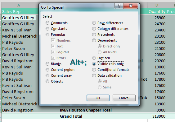
Visible Cells Only is available to add to the QAT. But you can't add it by right-clicking in the dialog box. To make matters worse, when you follow these steps, you have to look for a command called "Select Visible Cells" instead of a command called "Visible Cells Only".

1. Right-click anywhere in the Ribbon and choose Customize Quick Access Toolbar. The Excel Options dialog box opens showing a list of Popular Commands. I reject many of these popular commands because they are already a single-click on the Home tab of the Ribbon.

   

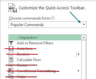
2. Open the drop-down menu to the right of Popular Commands and choose either All Commands or Commands Not In the Ribbon.
3. Scroll through the left list box to find the command.

   

4. Click the Add>> button in the center of the screen.

   

5. Click OK to close Excel Options.
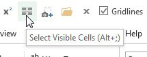
6. Hover over the newly added icon to see the tooltip and possibly learn of a keyboard shortcut.

   

Favorite QAT Icons From Twitter

If you are looking for something to make Twitter more interesting, consider following @MrExcel. You can then play along in fun surveys like this one:

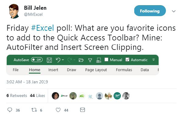
Presented below are several suggestions from people on Twitter.

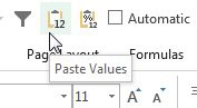
Thanks to ExcelCity, Adam Warrington, Dan Lanning, Christopher Broas. Bonus point to AJ Willikers who suggested both Paste Values and Paste Values and Number Formatting shown to the right of Paste Values above.

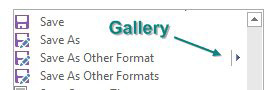
Sometimes, You Don't Want the Gallery

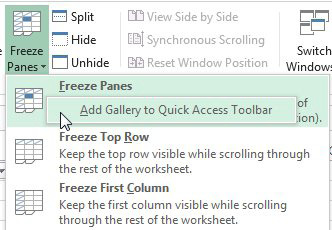
The next most popular command to add to the QAT is Freeze Panes. Go to the View tab. Open the Freeze Panes drop-down menu. Right-click on Freeze Panes and Excel offers "Add Gallery to the Quick Access Toolbar".

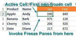
Freeze panes is a tricky command. If you want to freeze row 1 and columns A:B, you have to put the cell pointer in C2 before you invoke Freeze Panes.

Some people don't understand this, and in Excel 2007, the Excel team made the Freeze Panes gallery with choices to freeze top row and freeze first column for people who did not know to select C2 before invoking Freeze Panes.

Since you understand how Freeze Panes works, you don't want the gallery on the QAT. You just want the icon that does Freeze Panes.

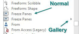
When you look for commands in the Excel Options, there are two choices for Freeze Panes. The one with the arrow is the gallery. The first one is the one you want.

Thanks to Debra Dalgleish, Colin Foster and @Excel_City for suggesting Freeze Panes

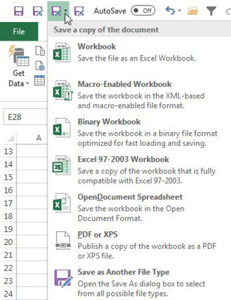
In other cases, the Gallery version is superior to the non-gallery version. Here is an example. Jen (who apparently is a @PFChangsAddict) suggested adding Save As to the QAT. Alex Waterton suggested adding Save As Other Formats. When I initially added the non-gallery version of Save As Other Formats, I realized that both icons open the Save As dialog box.

Instead, use the Gallery version of Save As

Here are those four icons in the QAT. The Save As Other Format gallery offers the most choices.

If you are planning on creating a lot of PDF files, Colin Foster suggests adding Publish as PDF or XPS to the QAT.

The First 9 Icons in QAT Have Easy Shortcut Keys

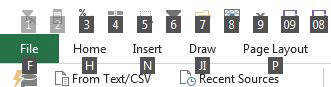
Most people who customize the QAT add new icons after the AutoSave, Save, Undo, Redo commands that are in the default QAT. But those first 9 QAT spots have super-easy keyboard shortcuts. AJ Willikers pointed out that the first 9 icons have easy short cut keys.

Press and release the Alt key. Key tips appear on each ribbon tab. So, Alt, H, S, O would sort descending. If you sort descending a lot, add the icon as one of the first 9 icons on the QAT. Press and release Alt, Then press 1 to invoke the first icon on the QAT. Note that the key tips for items 10 and beyond require you to press Alt, 0, 1 so they aren't quite as easy as the first 9 icons.

Thanks to AJ Willikers for pointing out the Alt 1-9 keyboard shortcuts.

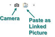
The Camera Tool versus Paste as Linked Picture

Another popular QAT command on Twitter was the Camera. This awesome hack dates back to Excel 97. It is great because it allows you to paste a live picture of cells from Sheet17 on the Dashboard worksheet. It was hard to use and Microsoft re-worked the tool in Excel 2007, rebranding it as Paste As Linked Picture. But the operation of the tool changed and some people like the old way better.

Old way: You could select the cells. Click the Camera icon. The mouse pointer changes to a cross hair. Click anywhere that you want to paste the picture of the cells.

New way: Copy the cells. Click in the new location. Choose Paste As Linked Picture. If you don't want the picture lined up with the top-left corner of the cell, drag to nudge the picture into position.

Screen Clipping to Capture a Static Image From Another Application

One of my favorite commands for the QAT is Insert Screen Clipping. Say that you want to grab a picture of a website and put it in your Excel worksheet. To effectively use the tool, you need to make sure that the web page is the most-recent window behind the Excel workbook. So - visit the web page. Then switch directly to your Excel Workbook. Choose Insert Screen Clipping and wait a few moments. The Excel screen disappears, revealing the web page. Wait for the web page to grey out, then use the mouse pointer to drag a rectangle around the portion of the web page. When you release the mouse button, a static picture of the web page (or any application) will paste in Excel. The Screen Clipping is also great for putting Excel charts in Power Point. Until you add this command to the QAT, it is hidden at the bottom of Insert, Screenshot. I don't like the Screenshot options because they put the entire full screen in Excel. Screen Clipping lets you choose just a part of the screen.

Two Icons Might Lead to the Same Place: Open Recent and Open

One of the popular QAT commands in Excel 2010 and Excel 2013 was the folder with a star - Open Recent File…. This command disappeared from Excel in Excel 2016. But people discovered that if you exported your settings from 2013 and then imported to 2016 or 2019, the icon would appear!

As I considered the prospect of dragging my Excel 2013 .tlb file around for the rest of my life, I inadvertently realized that the Open icon leads to the exact same place as the Open Recent File icon.

Clear Filter and Reapply Filter

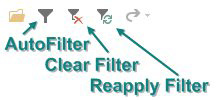
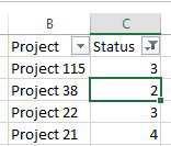
Bathazar Lawson suggests adding Reapply Filter to the QAT. Here is how this becomes handy. Let's say you have a list of projects. You don't need to see anything where the status code is Complete. You set up a filter for this.

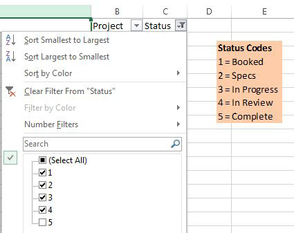
You change the status code on some projects. Some of the projects that used to be In Review are now Complete.

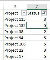
Instead of re-opening the Filter drop-down, click Reapply Filter.

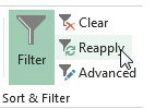
Excel will re-evaluate the data and hide the items which now have a 5.

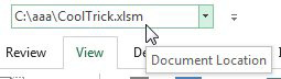
Some Future Features Debut on the QAT and then Become Real Features

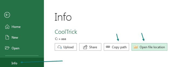
I was at a seminar in Topeka when Candace and Robert taught me that you could add an icon called Document Location to the QAT.

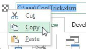
If you need to copy the document location to the clipboard, you can select the text from the QAT, right-click and choose Copy.

The Document Location has been available since at least Excel 2010. In early 2019, Office 365 subscribers will notice that the File, Info screen now has new equivalents of Copy Path and Open File Location.

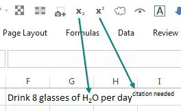
Easier Superscript and Subscripts

Add the new Superscript and Subscript icons to the QAT. As you are typing, click either icon to continue typing in subscript or superscript. This might be handy for a single character (such as the 2 in H20) or for several characters.

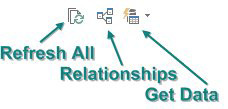
New Features from the Data Tab

The Data tab is like the Boardwalk and Park Place of the Excel ribbon. Every project manager wants to be on the Home tab, but most of the great features end up on the data tab. Excel 2016 introduced Get Data (Power Query), Relationships, and Refresh All. Add those to the QAT.

Build Formulas Without Ever Leaving the Mouse

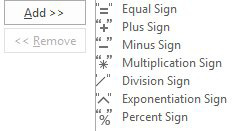
Ha-ha! This advice flies in the face of what every Excel tipster teaches. Most people want you to build formulas without ever leaving the keyboard. But what if you hate the keyboard and want to use the mouse? You can add these operators to your QAT:

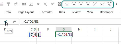
Using the mouse, you can click the Equals sign, then click on C1, then Multiply, then D1, then Divide, then E1. To complete the formula, click the green checkmark next to the formula bar to Enter. Surprisingly, Enter is not available for the QAT. But the formula bar is usually always visible, so this would work.

Those seven icons shown above are not located in one section of the Customize dialog. You have to hunt for them in the E, P, M, M, D, E, and P section of the list.

Show QAT Below the Ribbon

Right-click the Ribbon and choose Show Quick Access Toolbar Below The Ribbon. There are several advantages. First, it is a shorter mouse move to reach the icons. Second, when the QAT is above the Ribbon, you have less space until the icons run into the file name.

#evba #etipfree
📤You download App EVBA.info installed directly on the latest phone here : https://www.evba.info/p/app-evbainfo-setting-for-your-phone.html?m=1